The AUTOREG Procedure
- Overview
-
Getting Started

-
Syntax
-
DetailsMissing ValuesAutoregressive Error ModelAlternative Autocorrelation Correction MethodsGARCH ModelsHeteroscedasticity- and Autocorrelation-Consistent Covariance Matrix EstimatorGoodness-of-Fit Measures and Information CriteriaTestingPredicted ValuesOUT= Data SetOUTEST= Data SetPrinted OutputODS Table NamesODS Graphics
-
Examples
- References
One of the key assumptions of the ordinary regression model is that the errors have the same variance throughout the sample. This is also called the homoscedasticity model. If the error variance is not constant, the data are said to be heteroscedastic.
Since ordinary least squares regression assumes constant error variance, heteroscedasticity causes the OLS estimates to be inefficient. Models that take into account the changing variance can make more efficient use of the data. Also, heteroscedasticity can make the OLS forecast error variance inaccurate because the predicted forecast variance is based on the average variance instead of on the variability at the end of the series.
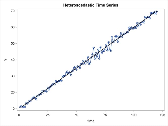
To illustrate heteroscedastic time series, the following statements create the simulated series Y. The variable Y has an error variance that changes from 1 to 4 in the middle part of the series.
data a;
   do time = -10 to 120;
      s = 1 + (time >= 60 & time < 90);
      u = s*rannor(12346);
      y = 10 + .5 * time + u;
      if time > 0 then output;
      end;
run;

title 'Heteroscedastic Time Series';
proc sgplot data=a noautolegend;
   series x=time y=y / markers;
   reg x=time y=y / lineattrs=(color=black);
run;
The simulated series is plotted in Figure 8.10.
To test for heteroscedasticity with PROC AUTOREG, specify the ARCHTEST option. The following statements regress Y on TIME and use the ARCHTEST= option to test for heteroscedastic OLS residuals:
/*-- test for heteroscedastic OLS residuals --*/
proc autoreg data=a;
   model y = time / archtest;
   output out=r r=yresid;
run;
The PROC AUTOREG output is shown in Figure 8.11. The Q statistics test for changes in variance across time by using lag windows that range from 1 through 12. (See the section Testing for Nonlinear Dependence: Heteroscedasticity Tests for details.) The p-values for the test statistics strongly indicate heteroscedasticity, with p < 0.0001 for all lag windows.
The Lagrange multiplier (LM) tests also indicate heteroscedasticity. These tests can also help determine the order of the ARCH model that is appropriate for modeling the heteroscedasticity, assuming that the changing variance follows an autoregressive conditional heteroscedasticity model.
Figure 8.11: Heteroscedasticity Tests
| Heteroscedastic Time Series |
| Dependent Variable | y |
|---|
| Ordinary Least Squares Estimates | |||
|---|---|---|---|
| SSE | 223.645647 | DFE | 118 |
| MSE | 1.89530 | Root MSE | 1.37670 |
| SBC | 424.828766 | AIC | 419.253783 |
| MAE | 0.97683599 | AICC | 419.356347 |
| MAPE | 2.73888672 | HQC | 421.517809 |
| Durbin-Watson | 2.4444 | Regress R-Square | 0.9938 |
| Total R-Square | 0.9938 | ||
| Tests for ARCH Disturbances Based on OLS Residuals | ||||
|---|---|---|---|---|
| Order | Q | Pr > Q | LM | Pr > LM |
| 1 | 19.4549 | <.0001 | 19.1493 | <.0001 |
| 2 | 21.3563 | <.0001 | 19.3057 | <.0001 |
| 3 | 28.7738 | <.0001 | 25.7313 | <.0001 |
| 4 | 38.1132 | <.0001 | 26.9664 | <.0001 |
| 5 | 52.3745 | <.0001 | 32.5714 | <.0001 |
| 6 | 54.4968 | <.0001 | 34.2375 | <.0001 |
| 7 | 55.3127 | <.0001 | 34.4726 | <.0001 |
| 8 | 58.3809 | <.0001 | 34.4850 | <.0001 |
| 9 | 68.3075 | <.0001 | 38.7244 | <.0001 |
| 10 | 73.2949 | <.0001 | 38.9814 | <.0001 |
| 11 | 74.9273 | <.0001 | 39.9395 | <.0001 |
| 12 | 76.0254 | <.0001 | 40.8144 | <.0001 |
| Parameter Estimates | |||||
|---|---|---|---|---|---|
| Variable | DF | Estimate | Standard Error |
t Value | Approx Pr > |t| |
| Intercept | 1 | 9.8684 | 0.2529 | 39.02 | <.0001 |
| time | 1 | 0.5000 | 0.003628 | 137.82 | <.0001 |
The tests of Lee and King (1993) and Wong and Li (1995) can also be applied to check the absence of ARCH effects. The following example shows that Wong and Li’s test is robust to detect the presence of ARCH effects with the existence of outliers.
/*-- data with outliers at observation 10 --*/
data b;
   do time = -10 to 120;
      s = 1 + (time >= 60 & time < 90);
      u = s*rannor(12346);
      y = 10 + .5 * time + u;
      if time = 10 then
         do; y = 200; end;
      if time > 0 then output;
   end;
run;
/*-- test for heteroscedastic OLS residuals --*/
proc autoreg data=b;
   model y = time / archtest=(qlm) ;
   model y = time / archtest=(lk,wl) ;
run;
As shown in Figure 8.12, the p-values of Q or LM statistics for all lag windows are above 90%, which fails to reject the null hypothesis of the absence of ARCH effects. Lee and King’s test, which rejects the null hypothesis for lags more than 8 at 10% significance level, works better. Wong and Li’s test works best, rejecting the null hypothesis and detecting the presence of ARCH effects for all lag windows.
Figure 8.12: Heteroscedasticity Tests
| Heteroscedastic Time Series |
| Tests for ARCH Disturbances Based on OLS Residuals | ||||
|---|---|---|---|---|
| Order | Q | Pr > Q | LM | Pr > LM |
| 1 | 0.0076 | 0.9304 | 0.0073 | 0.9319 |
| 2 | 0.0150 | 0.9925 | 0.0143 | 0.9929 |
| 3 | 0.0229 | 0.9991 | 0.0217 | 0.9992 |
| 4 | 0.0308 | 0.9999 | 0.0290 | 0.9999 |
| 5 | 0.0367 | 1.0000 | 0.0345 | 1.0000 |
| 6 | 0.0442 | 1.0000 | 0.0413 | 1.0000 |
| 7 | 0.0522 | 1.0000 | 0.0485 | 1.0000 |
| 8 | 0.0612 | 1.0000 | 0.0565 | 1.0000 |
| 9 | 0.0701 | 1.0000 | 0.0643 | 1.0000 |
| 10 | 0.0701 | 1.0000 | 0.0742 | 1.0000 |
| 11 | 0.0701 | 1.0000 | 0.0838 | 1.0000 |
| 12 | 0.0702 | 1.0000 | 0.0939 | 1.0000 |
| Tests for ARCH Disturbances Based on OLS Residuals | ||||
|---|---|---|---|---|
| Order | LK | Pr > |LK| | WL | Pr > WL |
| 1 | -0.6377 | 0.5236 | 34.9984 | <.0001 |
| 2 | -0.8926 | 0.3721 | 72.9542 | <.0001 |
| 3 | -1.0979 | 0.2723 | 104.0322 | <.0001 |
| 4 | -1.2705 | 0.2039 | 139.9328 | <.0001 |
| 5 | -1.3824 | 0.1668 | 176.9830 | <.0001 |
| 6 | -1.5125 | 0.1304 | 200.3388 | <.0001 |
| 7 | -1.6385 | 0.1013 | 238.4844 | <.0001 |
| 8 | -1.7695 | 0.0768 | 267.8882 | <.0001 |
| 9 | -1.8881 | 0.0590 | 304.5706 | <.0001 |
| 10 | -2.2349 | 0.0254 | 326.3658 | <.0001 |
| 11 | -2.2380 | 0.0252 | 348.8036 | <.0001 |
| 12 | -2.2442 | 0.0248 | 371.9596 | <.0001 |