The SSM Procedure (Experimental)
-
Overview

- Getting Started
-
Syntax
-
DetailsState Space Model and NotationTypes of Data OrganizationOverview of Model Specification SyntaxLikelihood, Filtering, and SmoothingContrasting PROC SSM with Other SAS Procedures Predefined Trend ModelsPredefined Structural ModelsCovariance ParameterizationMissing ValuesComputational IssuesDisplayed OutputODS Table NamesODS Graph NamesOUT= Data Set
-
ExamplesBivariate Basic Structural Model Two-Way Random-Effects and Autoregressive Model for Panel DataBackcasting, Forecasting, and InterpolationSmoothing of Repeated Measures DataA User-Defined Trend ModelModel with Multiple ARIMA ComponentsDynamic Factor ModelingDiagnostic PlotsVariable Bandwidth Smoothing
- References
This example provides information about the diagnostic plots that are produced by the SSM procedure. The following plots are available:
-
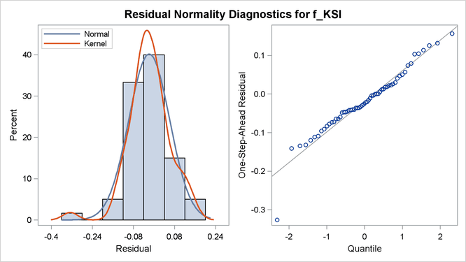
A panel of two plots—a histogram and a Q-Q plot—for the normality check of the one-step-ahead residuals
 . A separate panel is produced for each response variable.
-
A time series plot of standardized residuals, one per response variable.
-
A panel of two plots—a histogram and a Q-Q plot—for the normality check of the prediction errors
 . A separate panel is produced for each response variable.
-
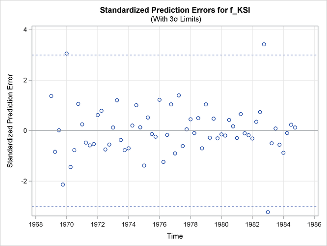
A time series plot of standardized prediction errors, one per response variable.
-
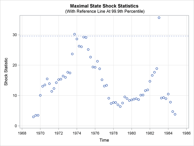
A time series plot of maximal state shock chi-square statistics.
All these plots are used primarily for model diagnostics. In this example the seat-belt data discussed in Example 27.1 are revisited. In Example 27.1 the question under consideration was whether the data showed evidence for the effectiveness of seat-belt law that was introduced
in the first quarter of 1983. An intervention variable, Q1_83_Shift, was used in the model to measure the effect of this law on the front-seat passengers who were killed or seriously injured
in the car accidents (f_KSI). Here the analysis of these data begins without the knowledge of this seat-belt law. In effect, the same model is fitted
without the use of the intervention variable Q1_83_Shift.
 proc ssm data=seatBelt optimizer(tech=interiorpoint) plots=all;
    id date interval=quarter;
    state error(2) type=WN cov(g);
    component wn1 = error[1];
    component wn2 = error[2];
    state level(2) type=RW cov(rank=1) ;
    component rw1 = level[1];
    component rw2 = level[2];
    state season(2) type=season(length=4);
    component s1 = season[1];
    component s2 = season[2];
    model f_KSI = rw1 s1  wn1;
    model r_KSI = rw2 s2 wn2;
 run;
The PLOTS=ALL option in the PROC SSM statement turns on all the plotting options. Since there are two response variables,
nine plots in total are produced: a separate set of four plots—two residual and two prediction error—is produced for f_KSI and r_KSI, and one maximal shock plot is produced. Only three of these plots are shown here. Output 27.8.1 shows the normality check for the one-step-ahead residuals for f_KSI. It shows some evidence of lack of normality.
Output 27.8.2 shows the time series plot of standardized prediction errors for f_KSI. It identifies some extreme observations (additive outliers): two near 1983 and one near 1970.
Output 27.8.3 shows the time series plot of maximal shock statistics. This plot can be very informative about the temporal locations of
the structural changes in the overall observation-generation process (treating the fitted model as the reference). It can
indicate locations of shifts in the process level or shifts in other characteristics such as its slope. The precise nature
of the shift (whether the shift is in the level or in some other aspects) must be determined by additional modeling steps
such as adding appropriate intervention variables to the model. In this example, the maximal shock statistics plot indicates
two locations—the last quarter of 1973 and the first quarter of 1983—as likely locations for the structural breaks that are
associated with the traffic accident process. These are indeed reasonable findings since the last quarter of 1973 (October
1973) is associated with the start of the oil shock that severely affected worldwide automobile traffic and the first quarter
of 1983 is associated with the introduction of the seat-belt law that might have improved the safety of front-seat passengers.
The following statements fit a revised model that includes the intervention variable Q1_83_Shift:
 proc ssm data=seatBelt optimizer(tech=interiorpoint) plots=all;
    id date interval=quarter;
    Q1_83_Shift = (date >= '1jan1983'd);
    state error(2) type=WN cov(g);
    component wn1 = error[1];
    component wn2 = error[2];
    state level(2) type=RW cov(rank=1) ;
    component rw1 = level[1];
    component rw2 = level[2];
    state season(2) type=season(length=4);
    component s1 = season[1];
    component s2 = season[2];
    model f_KSI = Q1_83_Shift rw1 s1  wn1;
    model r_KSI = rw2 s2 wn2;
 run;
Output 27.8.4 shows the time series plot of maximal shock statistics for this revised model. As expected, the plot no longer shows the first quarter of 1983 as a structural break location. It continues to show the last quarter of 1973 as a structural break location because the fitted model does not try to explicitly account for this shift.
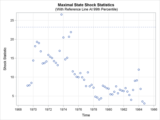
Note that the reference line in Output 27.8.3 is drawn at 99.9th percentile while the reference line in Output 27.8.4 is drawn at 99th percentile. The reference line location in the maximal state shock chi-square statistics plot is decided
based on the points in the plot. A reference line is drawn at percentiles 80, 90, 99, or 99.9 based on the largest maximal
shock statistic being shown.