The QLIM Procedure
- Overview
-
Getting Started

-
Syntax
-
DetailsOrdinal Discrete Choice ModelingLimited Dependent Variable ModelsStochastic Frontier Production and Cost ModelsHeteroscedasticity and Box-Cox TransformationBivariate Limited Dependent Variable ModelingSelection ModelsMultivariate Limited Dependent ModelsVariable SelectionTests on ParametersBayesian AnalysisPrior DistributionsOutput to SAS Data SetOUTEST= Data SetNamingODS Table NamesODS Graphics
-
Examples
- References
The PRIOR statement is used to specify the prior distribution of the model parameters. You must specify a list of parameters,
a tilde ![]() , and then a distribution with its parameters. You can specify multiple PRIOR statements to define independent priors. Parameters that are associated with a regressor variable are referred to by the
name of the corresponding regressor variable.
, and then a distribution with its parameters. You can specify multiple PRIOR statements to define independent priors. Parameters that are associated with a regressor variable are referred to by the
name of the corresponding regressor variable.
You can specify the special keyword _REGRESSORS to consider all the regressors of a model. If multiple prior statements affect the same parameter, the prior that is specified is used. For example, in a regression with three regressors (X1, X2, X3) the following statements imply that the prior on X1 is NORMAL(MEAN=0, VAR=1), the prior on X2 is GAMMA(SHAPE=3, SCALE=4), and the prior on X3 is UNIFORM(MIN=0, MAX=1):
...
prior _Regressors ~ uniform(min=0, max=1);
prior X1 X2 ~ gamma(shape=3, scale=4);
prior X1 ~ normal(mean=0, var=1);
...
If a parameter is not associated with a PRIOR statement or if some of the prior hyperparameters are missing, then the following default choices are considered:
Table 22.2: Default values for prior distributions.
|
PRIOR distribution |
|
|
|
|
|
|
NORMAL |
|
|
|
|
|
|
IGAMMA |
|
|
|
|
|
|
GAMMA |
|
|
|
|
|
|
UNIFORM |
|
|
|||
|
BETA |
|
|
|
|
|
|
T |
|
|
|
|
See the section Standard Distributions for density specification.
The choice of the prior distribution for a heteroscedastic model is particularly interesting. Based on the notation provided
in section HETERO Statement, you need to provide a prior for ![]() . This prior is enough to induce different
. This prior is enough to induce different ![]() into the analysis. The resulting inference is a compromise between two cases: the inference based on the entire sample and
the inference based on a single unit
into the analysis. The resulting inference is a compromise between two cases: the inference based on the entire sample and
the inference based on a single unit ![]() . The degree of compromise is determined by
. The degree of compromise is determined by ![]() .
.
This type of modeling is similar to a method called “hierarchical Bayes,” in which the prior is characterized by two levels:
one for each individual ![]() and one for the entire population
and one for the entire population ![]() . In this scenario the degree of compromise between the information provided by a unit and the information provided by the
entire sample is determined by the data.
. In this scenario the degree of compromise between the information provided by a unit and the information provided by the
entire sample is determined by the data.
The choice of the prior might not be straightforward, and it can heavily affect sampling performance. Depending on how the heteroscedastic effects are modeled, the default priors are
|
|
|
|
|
|
|
|
|
|
|
|
|
|
|
|
|
|
|
|
|
|
|
|
where ![]() ,
, ![]() , and
, and ![]() is a small number (by default,
is a small number (by default, ![]() for the EXPONENTIAL link function and
for the EXPONENTIAL link function and ![]() for the QUADRATIC link function).
for the QUADRATIC link function).
The priors for the EXPONENTIAL and QUADRATIC link functions are not straightforward. To understand the choices, do the following:
-
Assume that
![\[ \Strong{z}^{}_{i}{\bgamma }=z_{i1}{\gamma _1}+\ldots +z_{iJ}{\gamma _ J}\approx \bar{z}_{1}{\gamma _1}+\ldots +\bar{z}_{J}{\gamma _ J},\qquad \forall i \]](images/etsug_qlim0442.png)
-
Set the priors according to the link function type:
-
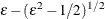
For the EXPONENTIAL link function, set
![$\displaystyle \textnormal{E}\left[\exp (\Strong{z}^{}_{i}{\bgamma })\right] $](images/etsug_qlim0443.png)

![$\displaystyle \textnormal{E}\left[\exp (\bar{z}_{1}{\gamma _1})\right]\times \ldots \times \textnormal{E}\left[\exp (\bar{z}_{J}{\gamma _ J})\right]=\varepsilon $](images/etsug_qlim0446.png)
![$\displaystyle \textnormal{V}\left[\exp (\Strong{z}^{}_{i}{\bgamma })\right] $](images/etsug_qlim0447.png)
![$\displaystyle \textnormal{E}\left[\exp (2\bar{z}_{1}{\gamma _1})\right]\times \ldots \times \textnormal{E}\left[\exp (2\bar{z}_{J}{\gamma _ J})\right]-\varepsilon ^2=1 $](images/etsug_qlim0448.png)
Assume a normal prior for
 , and set
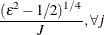
![$\displaystyle \textnormal{E}\left[\exp (\bar{z}_{j}{\gamma _ j})\right] $](images/etsug_qlim0450.png)


![$\displaystyle \textnormal{E}\left[\exp (2\bar{z}_{j}{\gamma _ j})\right] $](images/etsug_qlim0453.png)

Based on the properties of the lognormal distribution, the prior hyperparameters for
 can be derived. Notice that
  is the number of regressors that are used in the heterogeneous regression. If the intercept is excluded, then
  .
.
-
For the QUADRATIC link function, set
![$\displaystyle \textnormal{E}\left[(\Strong{z}^{}_{i}{\bgamma })^2\right] $](images/etsug_qlim0458.png)
![$\displaystyle \left[\textnormal{E}\left(\bar{z}_{1}{\gamma _1}+\ldots +\bar{z}_{J}{\gamma _ J}\right)\right]^2+\textnormal{V}\left[\bar{z}_{1}{\gamma _1}+\ldots +\bar{z}_{J}{\gamma _ J}\right]=\varepsilon $](images/etsug_qlim0460.png)
![$\displaystyle \textnormal{E}\left[(\bar{z}_{1}{\gamma _1}+\ldots +\bar{z}_{J}{\gamma _ J})^4\right]-\varepsilon ^2=1 $](images/etsug_qlim0461.png)
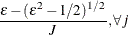
Assume a normal prior for
. Based on the properties of the normal distribution, the preceding expressions return
![$\displaystyle \textnormal{E}\left[\bar{z}_{1}{\gamma _1}+\ldots +\bar{z}_{J}{\gamma _ J}\right] $](images/etsug_qlim0462.png)

![$\displaystyle \textnormal{V}\left[\bar{z}_{1}{\gamma _1}+\ldots +\bar{z}_{J}{\gamma _ J}\right] $](images/etsug_qlim0465.png)


The prior hyperparameters for
can be derived by setting
![$\displaystyle \textnormal{E}\left[\bar{z}_{j}{\gamma _ j}\right] $](images/etsug_qlim0470.png)
![$\displaystyle \textnormal{V}\left[\bar{z}_{j}{\gamma _ j}\right] $](images/etsug_qlim0473.png)
Notice that
is the number of regressors that are used in the heterogeneous regression. If the intercept is excluded, then . It is important to emphasize that the restriction  is likely to introduce some distortion because
  cannot be any “small” number.
-
Table 22.3 through Table 22.8 show all the distribution density functions that PROC QLIM recognizes. You specify these distribution densities in the PRIOR statement.
![$ \left\{ \begin{array}{ll} \left[ m, M \right] & \mbox{when } a = 1, b = 1 \\ \left[ m, M \right) & \mbox{when } a = 1, b \neq 1 \\ \left( m, M \right] & \mbox{when } a \neq 1, b = 1 \\ \left( m, M \right) & \mbox{otherwise} \end{array} \right. $](images/etsug_qlim0482.png)
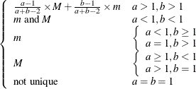
Table 22.4: Gamma Distribution
|
PRIOR statement |
GAMMA(SHAPE= |
|
Density |
|
|
Parameter restriction |
|
|
Range |
|
|
Mean |
|
|
Variance |
|
|
Mode |
|
|
Defaults |
SHAPE=SCALE=1 |
Table 22.5: Inverse-Gamma Distribution
|
PRIOR statement |
IGAMMA(SHAPE= |
|
Density |
|
|
Parameter restriction |
|
|
Range |
|
|
Mean |
|
|
Variance |
|
|
Mode |
|
|
Defaults |
SHAPE=2.000001, SCALE=1 |
Table 22.6: Normal Distribution
|
PRIOR statement |
NORMAL(MEAN= |
|
Density |
|
|
Parameter restriction |
|
|
Range |
|
|
Mean |
|
|
Variance |
|
|
Mode |
|
|
Defaults |
MEAN=0, VAR=1000000 |
Table 22.7: ![]() Distribution
Distribution
|
PRIOR statement |
T(LOCATION= |
|
Density |
|
|
Parameter restriction |
|
|
Range |
|
|
Mean |
|
|
Variance |
|
|
Mode |
|
|
Defaults |
LOCATION=0, DF=3 |
Table 22.8: Uniform Distribution
|
PRIOR statement |
UNIFORM(MIN= |
|
Density |
|
|
Parameter restriction |
|
|
Range |
|
|
Mean |
|
|
Variance |
|
|
Mode |
Not unique |
|
Defaults |
MIN |