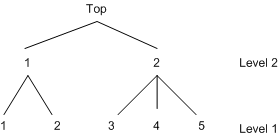
Decision Tree and Nested Logit :: SAS/ETS(R) 12.3 User's Guide

Decision Tree and Nested Logit

You can view choices as a decision tree and model the decision tree by using the nested logit model. You need to use either the NEST statement or the CHOICE= option of the MODEL statement to specify the nested tree structure. Additionally, you need to identify which explanatory variables are used at each level of the decision tree. These explanatory variables are arguments for what is called a utility function. The utility function is specified using UTILITY statements. For example, consider a two-level decision tree. The tree structure is displayed in Figure 18.27.

Figure 18.27: Two-Level Decision Tree

A nested logit model with two levels can be specified using the following SAS statements:

   proc mdc data=one type=nlogit;
      model decision = x1 x2 x3 x4 x5 /
            choice=(upmode 1 2, mode 1 2 3 4 5);
      id pid;
      utility u(1, 3 4 5 @ 2) = x1 x2,
              u(1, 1 2 @ 1) = x3 x4,
              u(2, 1 2) = x5;
   run;

The DATA=one data set should be arranged as follows:

   obs  pid  upmode   mode   x1  x2  x3  x4  x5  decision
    1    1     1       1     #   #   #   #   #      1
    2    1     1       2     #   #   #   #   #      0
    3    1     2       3     #   #   #   #   #      0
    4    1     2       4     #   #   #   #   #      0
    5    1     2       5     #   #   #   #   #      0
    6    2     1       1     #   #   #   #   #      0
    7    2     1       2     #   #   #   #   #      0
    8    2     2       3     #   #   #   #   #      0
    9    2     2       4     #   #   #   #   #      0
   10    2     2       5     #   #   #   #   #      1

All model variables, x1 through x5, are specified in the UTILITY statement. It is required that entries denoted as # have values for model estimation and prediction. The values of the level 2 utility variable x5 should be the same for all the primitive (level 1) alternatives below node 1 at level 2 and, similarly, for all the primitive alternatives below node 2 at level 2. In other words, x5 should have the same value for primitive alternatives 1 and 2 and, similarly, it should have the same value for primitive alternatives 3, 4, and 5. More generally, the values of any level 2 or higher utility function variables should be constant across primitive alternatives under each node for which the utility function applies. Since PROC MDC expects this to be the case, it uses the values of x5 only for the primitive alternatives 1 and 3, ignoring the values for the primitive alternatives 2, 4, and 5. Thus, PROC MDC uses the values of the utility function variable only for the primitive alternatives that come first under each node for which the utility function applies. This behavior applies to any utility function variables that are specified above the first level. The choice variable for level 2 (upmode ) should be placed before the first-level choice variable (mode ) when the CHOICE= option is specified. Alternatively, the NEST statement can be used to specify the decision tree. The following SAS statements fit the same nested logit model:

   proc mdc data=a type=nlogit;
      model decision = x1 x2 x3 x4 x5 /
               choice=(mode 1 2 3 4 5);
      id pid;
      utility u(1, 3 4 5 @ 2) = x1 x2,
              u(1, 1 2 @ 1) = x3 x4,
              u(2, 1 2) = x5;
      nest level(1) = (1 2 @ 1, 3 4 5 @ 2),
           level(2) = (1 2 @ 1);
   run;

The U(1, 3 4 5 @ 2)= option specifies three choices, 3, 4, and 5, at level 1 of the decision tree. They are connected to the upper branch 2. The specified variables (x1 and x2) are used to model this utility function. The bottom level of the decision tree is level 1. All variables in the UTILITY statement must be included in the MODEL statement. When all choices at the first level share the same variables, you can omit the second argument of the U()= option for that level. However, U(1, ) = x1 x2 is not equivalent to the following statements:

   u(1, 3 4 5 @ 2) = x1 x2;
   u(1, 1 2 @ 1) = x1 x2;

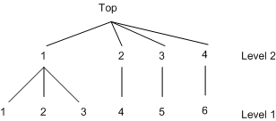
The CHOICE= variables need to be specified from the top to the bottom level. To forecast demand for new products, stated preference data are widely used. Stated preference data are attractive for market researchers because attribute variations can be controlled. Hensher (1993) explores the advantage of combining revealed preference (market data) and stated preference data. The scale factor ( $\Variable{V}_{rp}/\Variable{V}_{sp}$ ) can be estimated using the nested logit model with the decision tree structure displayed in Figure 18.28.

Figure 18.28: Decision Tree for Revealed and Stated Preference Data

Example SAS statements are as follows:

   proc mdc data=a type=nlogit;
      model decision = x1 x2 x3 /
               spscale
               choice=(mode 1 2 3 4 5 6);
      id pid;
      utility u(1,) = x1 x2 x3;
      nest level(1) = (1 2 3 @ 1, 4 @ 2, 5 @ 3, 6 @ 4),
           level(2) = (1 2 3 4 @ 1);
   run;

The SPSCALE option specifies that parameters of inclusive values for nodes 2, 3, and 4 at level 2 be the same. When you specify the SAMESCALE option, the MDC procedure imposes the same coefficient of inclusive values for choices 1–4.