The TIMESERIES Procedure
- Overview
- Getting Started
-
Syntax

-
DetailsAccumulationMissing Value InterpretationTime Series TransformationTime Series DifferencingDescriptive StatisticsSeasonal DecompositionCorrelation AnalysisCross-Correlation AnalysisSpectral Density AnalysisSingular Spectrum AnalysisData Set OutputOUT= Data SetOUTCORR= Data SetOUTCROSSCORR= Data SetOUTDECOMP= Data SetOUTPROCINFO= Data SetOUTSEASON= Data SetOUTSPECTRA= Data SetOUTSSA= Data SetOUTSUM= Data SetOUTTREND= Data Set_STATUS_ Variable ValuesPrinted OutputODS Table NamesODS Graphics Names
-
Examples
- References
Spectral Density Analysis
Spectral analysis can be performed on the working series by specifying the OUTSPECTRA= option or by specifying the PLOTS=PERIODOGRAM
or PLOTS=SPECTRUM option in the PROC TIMESERIES statement. PROC TIMESERIES uses the finite Fourier transform to decompose
data series into a sum of sine and cosine terms of different amplitudes and wavelengths. The finite Fourier transform decomposition
of the series ![]() is
is
|
|
|
|
|
|
where

-
is the time subscript,

-
are the equally spaced time series data

-
is the number of observations in the time series

-
is the number of frequencies in the Fourier decomposition:
 if is even,
  if is odd

-
is the frequency subscript,

-
is the mean term:


-
are the cosine coefficients

-
are the sine coefficients

-
are the Fourier frequencies:

The Fourier decomposition is performed after the ACCUMULATE=, DIF=, SDIF= and TRANSFORM= options in the ID and VAR statements have been applied.
Functions of the Fourier coefficients ![]() and
and ![]() can be plotted against frequency or against wavelength to form periodograms. The amplitude periodogram
can be plotted against frequency or against wavelength to form periodograms. The amplitude periodogram ![]() is defined as follows:
is defined as follows:
|
|
Since the Fourier transform is an even, periodic function of frequency which repeats every ![]() ordinates the periodogram is also. Values of
ordinates the periodogram is also. Values of ![]() for all
for all ![]() therefore can be mapped to the unique values
therefore can be mapped to the unique values ![]() using the equations
using the equations
|
|
|
|
|
|
|
|
|
|
|
|
|
|
|
The periodogram, ![]() , is an estimate at the discrete frequencies
, is an estimate at the discrete frequencies ![]() of the spectral density function which characterizes the series
of the spectral density function which characterizes the series ![]() . By smoothing the periodogram an improved spectral density estimate with reduced variance and bias can be achieved at these
points. Smoothing can be accomplished either through use of a spectral window smoothing function or by applying a lag window
filter to the series autocovariance function.
. By smoothing the periodogram an improved spectral density estimate with reduced variance and bias can be achieved at these
points. Smoothing can be accomplished either through use of a spectral window smoothing function or by applying a lag window
filter to the series autocovariance function.
When the SPECTRA statement’s DOMAIN=FREQUENCY option is in effect spectral density estimates are computed by smoothing the periodogram ordinates using the equation
|
|
where ![]() is the spectral window function whose form is specified by either the KERNEL= option or the WEIGHTS option.
is the spectral window function whose form is specified by either the KERNEL= option or the WEIGHTS option. ![]() is the kernel scale parameter which acts as a frequency scaling factor in the spectral window smoothing function. Values
of
is the kernel scale parameter which acts as a frequency scaling factor in the spectral window smoothing function. Values
of ![]() that fall outside of
that fall outside of ![]() are mapped to values inside this range by the equations presented previously.
are mapped to values inside this range by the equations presented previously.
When the DOMAIN=TIME option is specified spectral density values are estimated by applying a lag window filter, ![]() , to the series autocovariance function. The spectral density estimate then can be computed from the filtered autocovariance
function using the equation
, to the series autocovariance function. The spectral density estimate then can be computed from the filtered autocovariance
function using the equation
|
|
In this case the kernel scale parameter, ![]() , serves as a scale factor for the lag length,
, serves as a scale factor for the lag length, ![]() , in the time domain. In the lag window formulation the spectral density estimate is a consistent estimator as
, in the time domain. In the lag window formulation the spectral density estimate is a consistent estimator as ![]() under the conditions
under the conditions ![]() for
for ![]() , and
, and ![]() . These conditions lead to the following parameterization of
. These conditions lead to the following parameterization of ![]() provided by the SPECTRA statement:
provided by the SPECTRA statement:
|
|
where the values ![]() and
and ![]() satisfy the consistency conditions. To specify the kernel scale parameter explicitly, set
satisfy the consistency conditions. To specify the kernel scale parameter explicitly, set ![]() to the desired scale factor and
to the desired scale factor and ![]() .
.
For uniformity and computational efficiency all spectral density estimates are calculated using a spectral window weighting
function, ![]() , applied to the periodogram ordinates. In the case where the DOMAIN=TIME option is specified the effective spectral window
weighting function is computed by the equation
, applied to the periodogram ordinates. In the case where the DOMAIN=TIME option is specified the effective spectral window
weighting function is computed by the equation
|
|
Because the kernel scale parameter, ![]() , serves as a lag scale factor in the time domain and bandwidth scale factor in the frequency domain the impact of
, serves as a lag scale factor in the time domain and bandwidth scale factor in the frequency domain the impact of ![]() on spectral density estimates depends on the value of the DOMAIN= option. When DOMAIN=FREQUENCY increasing values of
on spectral density estimates depends on the value of the DOMAIN= option. When DOMAIN=FREQUENCY increasing values of ![]() decrease variance and increase bias in the spectral density estimates whereas when DOMAIN=TIME increasing values of
decrease variance and increase bias in the spectral density estimates whereas when DOMAIN=TIME increasing values of ![]() increase variance and decrease bias.
increase variance and decrease bias.
Using Kernel Specifications
You can specify one of ten different kernel smoothing functions in the SPECTRA statement. Five smoothing functions are available as KERNEL= options and five complementary smoothing functions which correspond to lag window filters are available when the KERNEL= option is used in conjunction with the DOMAIN=TIME option.
For example, a Parzen kernel with a support of 11 periodogram ordinates in the frequency domain can be specified using the kernel option:
spectra / parzen c=5 expon=0;
The TIMESERIES procedure supports the following spectral window kernel functions in the frequency domain where ![]() :
:
BARTLETT: Bartlett kernel
|
|
|
|
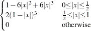
PARZEN: Parzen kernel
|
|
|
 |
QS: quadratic spectral kernel
|
|
|
|
TUKEY: Tukey-Hanning kernel
|
|
|
|
TRUNCAT: truncated kernel
|
|
|
|
When the DOMAIN=TIME option is specified the five kernel functions above are interpreted as lag window filters on the autocovariance
function. The lag window kernel functions correspond to the following spectral window smoothing functions where ![]() :
:
BARTLETT: Bartlett equivalent lag window filter
|
|
|
|
PARZEN: Parzen equivalent lag window filter
|
|
|
|
QS: quadratic spectral equivalent lag window filter
|
|
|
|
TUKEY: Tukey-Hanning equivalent lag window filter
|
|
|
|
|
|
|
|
TRUNC: truncated equivalent lag window filter
|
|
|
|
Using Specification of Weight Constants
Any number of weighting constants can be specified. The constants are interpreted symmetrically about the middle weight. The middle constant (or the constant to the right of the middle if an even number of weight constants is specified) is the relative weight of the current periodogram ordinate. The constant immediately following the middle one is the relative weight of the next periodogram ordinate, and so on. The actual weights used in the smoothing process are the weights specified in the WEIGHTS option scaled so that they sum to 1.
The moving average calculation reflects at each end of the periodogram to accommodate the periodicity of the periodogram function.
For example, a simple triangular weighting can be specified using the following WEIGHTS option:
spectra / weights 1 2 3 2 1;
Computational Method
If the number of observations, ![]() , factors into prime integers that are less than or equal to 23, and the product of the square-free factors of
, factors into prime integers that are less than or equal to 23, and the product of the square-free factors of ![]() is less than 210, then the procedure uses the fast Fourier transform developed by Cooley and Tukey (1965) and implemented
by Singleton (1969). If
is less than 210, then the procedure uses the fast Fourier transform developed by Cooley and Tukey (1965) and implemented
by Singleton (1969). If ![]() cannot be factored in this way, then the procedure uses a Chirp-Z algorithm similar to that proposed by Monro and Branch
(1976).
cannot be factored in this way, then the procedure uses a Chirp-Z algorithm similar to that proposed by Monro and Branch
(1976).
Missing Values
Missing values are replaced with an estimate of the mean to perform spectral analyses. This treatment of a series with missing values is consistent with the approach used by Priestley (1981).