The TCOUNTREG Procedure (Experimental)
- Overview
- Getting Started
-
Syntax

-
Details
 Specification of RegressorsMissing ValuesPoisson RegressionNegative Binomial RegressionZero-Inflated Count Regression OverviewZero-Inflated Poisson RegressionZero-Inflated Negative Binomial RegressionVariable SelectionPanel Data AnalysisComputational ResourcesNonlinear Optimization OptionsCovariance Matrix TypesDisplayed OutputOUTPUT OUT= Data SetOUTEST= Data SetODS Table NamesODS Graphics
 -
Examples

- References
Example 30.1 Basic Models
Data Description and Objective
The data set docvisit contains information for approximately 5,000 Australian individuals about the number and possible determinants of doctor
visits that were made during a two-week interval. This data set contains a subset of variables taken from the Racd3 data set used by Cameron and Trivedi (1998). The docvisit data set can be found in the SAS/ETS Sample Library.
The variable doctorco represents doctor visits. Additional variables in the data set that you want to evaluate as determinants of doctor visits
include sex (coded 0=male, 1=female), age (age in years divided by 100), illness (number of illnesses during the two-week interval, with five or more coded as five), income (annual income in Australian dollars divided by 1,000), and hscore (a general health questionnaire score, where a high score indicates bad health). Summary statistics for these variables are
computed in the following statements and presented in Output 30.1.1.
proc means data=docvisit;
   var doctorco sex age illness income hscore;
run;
Output 30.1.1: Summary Statistics
| Variable | N | Mean | Std Dev | Minimum | Maximum | ||||||||||||||||||||||||||||||||||||
|---|---|---|---|---|---|---|---|---|---|---|---|---|---|---|---|---|---|---|---|---|---|---|---|---|---|---|---|---|---|---|---|---|---|---|---|---|---|---|---|---|---|
|
|
|
|
|
|
Poisson Model
The following statements fit a Poisson model to the data by using the covariates SEX, ILLNESS, INCOME, and HSCORE:
proc tcountreg data=docvisit plots(only counts(0 to 4 by 1))=(predprob predpro);
   model doctorco=sex illness income hscore / dist=poisson printall;
run;
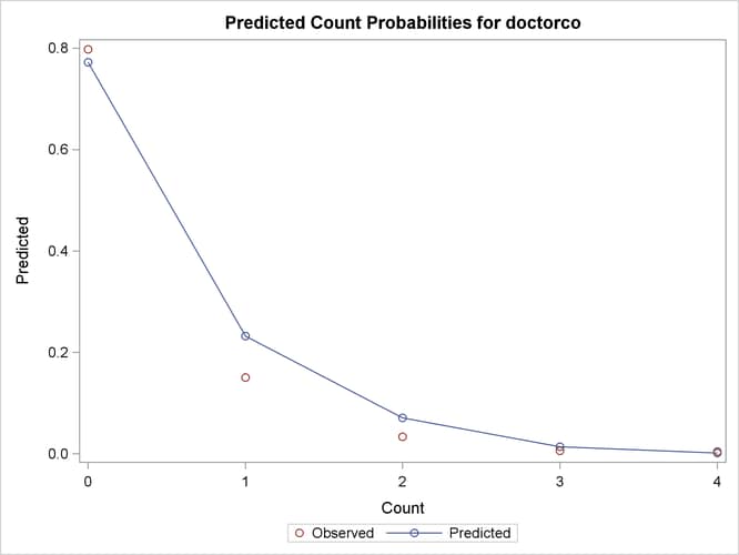
Output 30.1.2: Mean Predicted Count Probabilities

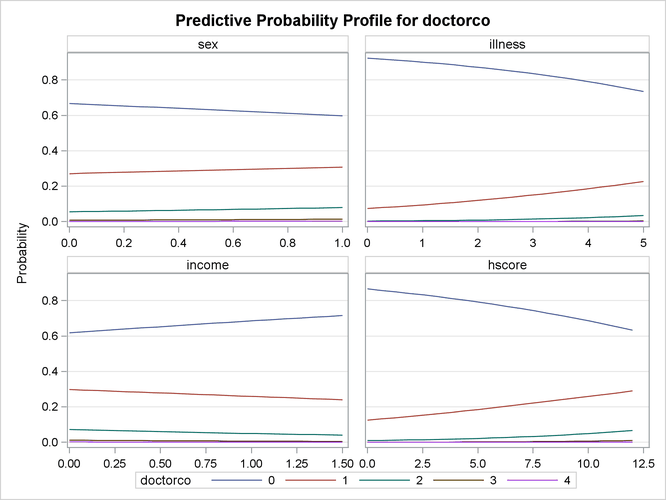
Output 30.1.2 shows the predicted frequencies of count levels 0 to 4 from the Poisson model. Although most of the observed counts would appear to be in the range 0 to 4, in fact observed counts between 0 and 4 account for more than 99% of the entire data set. One thing that would be interesting to explore is how the model-predicted probabilities of those count levels react to different regressor values. Output 30.1.3 shows the predictive profiles of the count levels in question against the first three regressors in the model. In each panel, the regressor in question is varied while all other regressors are fixed at their observed mean and the model parameters are fixed at their MLE.
Output 30.1.3: Profile Function of Predictive Probabilities

In this example, the DIST= option in the MODEL statement specifies the POISSON distribution. In addition, the PRINTALL option displays the correlation and covariance matrices for the parameters, log-likelihood values, and convergence information in addition to the parameter estimates. The parameter estimates for this model are shown in Output 30.1.4.
Output 30.1.4: Parameter Estimates of Poisson Model
| Parameter Estimates | |||||
|---|---|---|---|---|---|
| Parameter | DF | Estimate | Standard Error | t Value | Approx Pr > |t| |
| Intercept | 1 | -1.855552 | 0.074545 | -24.89 | <.0001 |
| sex | 1 | 0.235583 | 0.054362 | 4.33 | <.0001 |
| illness | 1 | 0.270326 | 0.017080 | 15.83 | <.0001 |
| income | 1 | -0.242095 | 0.077829 | -3.11 | 0.0019 |
| hscore | 1 | 0.096313 | 0.009089 | 10.60 | <.0001 |
Using the CLASS statement
If some regressors are categorical in nature (meaning that these variables can take only a few discrete qualitative values), specify them in the CLASS statement. In this example, SEX is categorical because it takes only two values. A class variable can be numeric or character.
Consider the following extension:
proc tcountreg data=docvisit;
   class sex;
   model doctorco=sex illness income hscore / dist=poisson;
run;
The partial output is given in Output 30.1.5.
Output 30.1.5: Parameter Estimates of Poisson Model with CLASS statement
| Parameter Estimates | |||||
|---|---|---|---|---|---|
| Parameter | DF | Estimate | Standard Error | t Value | Approx Pr > |t| |
| Intercept | 1 | -1.619969 | 0.063985 | -25.32 | <.0001 |
| sex 0 | 1 | -0.235583 | 0.054362 | -4.33 | <.0001 |
| sex 1 | 0 | 0 | . | . | . |
| illness | 1 | 0.270326 | 0.017080 | 15.83 | <.0001 |
| income | 1 | -0.242095 | 0.077829 | -3.11 | 0.0019 |
| hscore | 1 | 0.096313 | 0.009089 | 10.60 | <.0001 |
If the CLASS statement is present, the TCOUNTREG procedure creates as many indicator or dummy variables as there are categories
in a class variable and uses them as independent variables. In order to avoid collinearity with the intercept, the last-created
dummy variable is assigned a zero coefficient by default. This means that only the dummy variable that is associated with
the first level of sex (male=0) is used as a regressor. Consequently, the estimated coefficient for this dummy variable is
the negative of the one for the original SEX variable in Output 30.1.4 because the reference level has switched from male to female.
Now consider a more practical task. The previous example implicitly assumed that each additional illness during the two-week interval has the same effect. In other words, this variable was thought of as a continuous variable. But this variable has only six values, and it is quite possible that the number of illnesses has a nonlinear effect on doctor visits. In order to check this conjecture, the following statements specify ILLNESS in the CLASS statement so that it is represented in the model by a set of six dummy variables that can account for any type of nonlinearity:
proc tcountreg data=docvisit;
   class sex illness;
   model doctorco=sex illness income hscore / dist=poisson;
run;
The parameter estimates are displayed in Output 30.1.6.
Output 30.1.6: Parameter Estimates of Poisson Model with CLASS statement
| Parameter Estimates | |||||
|---|---|---|---|---|---|
| Parameter | DF | Estimate | Standard Error | t Value | Approx Pr > |t| |
| Intercept | 1 | -0.385930 | 0.088062 | -4.38 | <.0001 |
| sex 0 | 1 | -0.219118 | 0.054190 | -4.04 | <.0001 |
| sex 1 | 0 | 0 | . | . | . |
| illness 0 | 1 | -1.934983 | 0.121267 | -15.96 | <.0001 |
| illness 1 | 1 | -0.698307 | 0.089732 | -7.78 | <.0001 |
| illness 2 | 1 | -0.471100 | 0.090742 | -5.19 | <.0001 |
| illness 3 | 1 | -0.488481 | 0.099127 | -4.93 | <.0001 |
| illness 4 | 1 | -0.272372 | 0.107593 | -2.53 | 0.0114 |
| illness 5 | 0 | 0 | . | . | . |
| income | 1 | -0.253583 | 0.077441 | -3.27 | 0.0011 |
| hscore | 1 | 0.094590 | 0.009025 | 10.48 | <.0001 |
Each ILLNESS parameter in this model represents the difference between each effect of ILLNESS and ILLNESS=5. Note that these estimates for different ILLNESS categories do not increase linearly, but instead show a relatively large jump from zero illnesses to one followed by relatively smaller increases.
Zero-Inflated Poisson model
Suppose that you suspect that the population of individuals can be viewed as two distinct groups: a low-risk group, consisting of individuals who never go to the doctor, and a high-risk group, consisting of individuals who do go to the doctor. You might suspect that the data have this structure both because the sample variance of DOCTORCO (0.64) exceeds its sample mean (0.30), which suggests overdispersion, and also because a large fraction of the DOCTORCO observations (80%) have the value zero. Estimating a zero-inflated model is one way to deal with overdispersion that results from excess zeros.
Suppose also that you suspect that the covariate AGE has an impact on whether an individual belongs to the low-risk group.
For example, younger individuals might have illnesses of much lower severity when they do get sick and be less likely to visit
a doctor, all else being equal. The following statements estimate a zero-inflated Poisson regression with AGE as a covariate in the zero-generation process:
proc tcountreg data=docvisit plots(only)=(dispersion zeroprofile);
   model doctorco=sex illness income hscore / dist=zip;
   zeromodel doctorco ~ age;
run;
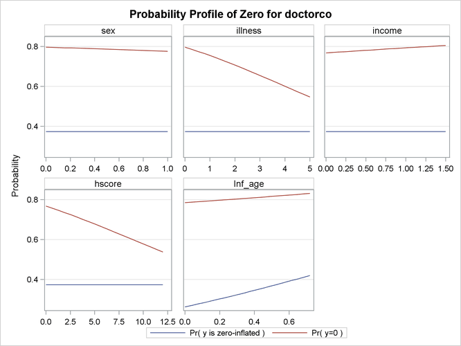
Output 30.1.7: Profile Function of Zero Process Selection and Zero Prediction

You might be interested in exploring how the zero process selection probability reacts to different regressor values. Output 30.1.7 displays this information in much the same fashion as Output 30.1.3. Since sex, illness, income, and hscore do not appear in the ZEROMODEL statement, the zero-inflation selection probability does not change for different values of
those regressors. However, the plot shows that age positively affects the zero process selection probability in a linear fashion.
In this case, the ZEROMODEL statement that follows the MODEL statement specifies that both an intercept and the variable AGE be used to estimate the likelihood of zero doctor visits. Output 30.1.8 shows the resulting parameter estimates.
Output 30.1.8: Parameter Estimates for ZIP Model
| Parameter Estimates | |||||
|---|---|---|---|---|---|
| Parameter | DF | Estimate | Standard Error | t Value | Approx Pr > |t| |
| Intercept | 1 | -1.033387 | 0.096973 | -10.66 | <.0001 |
| sex | 1 | 0.122511 | 0.062566 | 1.96 | 0.0502 |
| illness | 1 | 0.237478 | 0.019997 | 11.88 | <.0001 |
| income | 1 | -0.143945 | 0.087810 | -1.64 | 0.1012 |
| hscore | 1 | 0.088386 | 0.010043 | 8.80 | <.0001 |
| Inf_Intercept | 1 | 0.986557 | 0.131339 | 7.51 | <.0001 |
| Inf_age | 1 | -2.090923 | 0.270580 | -7.73 | <.0001 |
The estimates of the zero-inflated intercept (Inf_Intercept) and the zero-inflated regression coefficient for AGE (Inf_age) are approximately 0.99 and –2.09, respectively. Since the zero-inflation model uses a logistic link by default, you can estimate the probabilities for individuals of ages 20, 50, and 70 as follows:
|
|
|
|
|
|
|
|
|
|
|
|
That is, the estimated probability of belonging to the low-risk group is about 0.64 for a 20-year-old individual, 0.49 for a 50-year-old individual, and only 0.38 for a 70-year-old individual. This supports the suspicion that older individuals are more likely to have a positive number of doctor visits.
Alternative models to account for the overdispersion are the negative binomial and the zero-inflated negative binomial models, which can be fit using the DIST=NEGBIN and DIST=ZINB options, respectively.
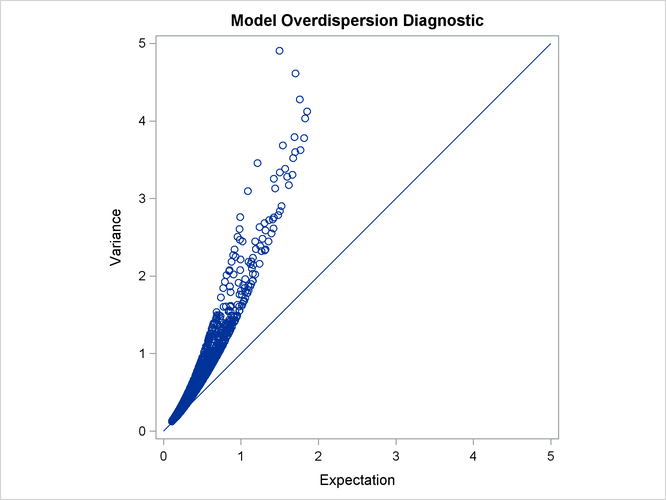
Output 30.1.9: Over-dispersion Diagnostic Plot

Output 30.1.9 plots the conditional variance against the conditional mean and can be used as a diagnostic tool to check the level of overdispersion in a model.