The QLIM Procedure
- Overview
-
Getting Started

-
Syntax
-
DetailsOrdinal Discrete Choice ModelingLimited Dependent Variable ModelsStochastic Frontier Production and Cost ModelsHeteroscedasticity and Box-Cox TransformationBivariate Limited Dependent Variable ModelingSelection ModelsMultivariate Limited Dependent ModelsVariable SelectionTests on ParametersBayesian AnalysisPrior DistributionsOutput to SAS Data SetOUTEST= Data SetNamingODS Table NamesODS Graphics
-
Examples
- References
Example 22.8 Bayesian Modeling
This example illustrates how to use the QLIM procedure to perform Bayesian analysis. The generated data mimic a hypothetic scenario in which you study the number of tickets sold for a sports event given the probability of the hosting team winning and the price of the tickets. The following statements create the dataset:
title1 'Bayesian Analysis';

ods graphics on;

data test;
   do i=1 to 200;
      e1 = rannor(8726)*2000;
      WinChance = ranuni(8772);
      Price = 10+ranexp(8773)*4;
      y = 48000 + 5000*WinChance - 100 * price +  e1;
      if y>50000 then TicketSales = 50000;
      if y<=50000 then TicketSales = y;
      output;
   end;
   keep WinChance price  y TicketSales;
run;
The following statements perform Bayesian analysis of a Tobit model:
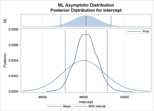
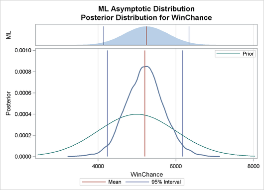
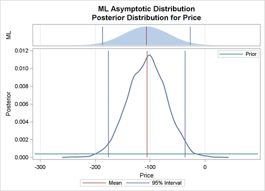
proc qlim data=test plots(prior)=all;
   model TicketSales = WinChance price;
   endogenous TicketSales ~ censored(lb=0 ub= 50000);
   prior intercept~normal(mean=48000);
   prior WinChance~normal(mean=5000);
   prior Price~normal(mean=-100);
   bayes NBI=10000 NMC=30000 THIN=1 ntrds=1 DIAG=ALL STATS=ALL seed=2;
run;
Output 22.8.1 shows the results from the maximum likelihood estimation and the Bayesian analysis with diffuse prior of this Tobit model.
Output 22.8.1: Bayesian Tobit Model
| Bayesian Analysis |
| Parameter Estimates | |||||
|---|---|---|---|---|---|
| Parameter | DF | Estimate | Standard Error | t Value | Approx Pr > |t| |
| Intercept | 1 | 48119 | 623.565045 | 77.17 | <.0001 |
| WinChance | 1 | 5242.083501 | 559.151222 | 9.38 | <.0001 |
| Price | 1 | -106.731665 | 40.660795 | -2.62 | 0.0087 |
| _Sigma | 1 | 1939.607206 | 134.348772 | 14.44 | <.0001 |
| Posterior Summaries | ||||||
|---|---|---|---|---|---|---|
| Parameter | N | Mean | Standard Deviation |
Percentiles | ||
| 25% | 50% | 75% | ||||
| Intercept | 30000 | 48123.2 | 525.7 | 47770.8 | 48122.3 | 48475.2 |
| WinChance | 30000 | 5201.8 | 487.2 | 4878.6 | 5202.9 | 5516.6 |
| Price | 30000 | -105.4 | 35.6176 | -129.5 | -104.6 | -81.2673 |
| _Sigma | 30000 | 1946.1 | 136.0 | 1852.0 | 1934.4 | 2032.7 |
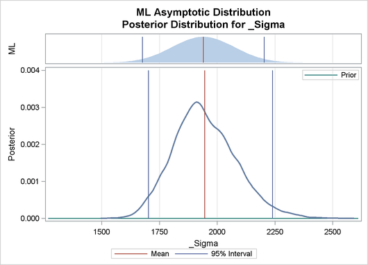
Output 22.8.2 depicts a graphical representation of MLE, prior, and posterior distributions.
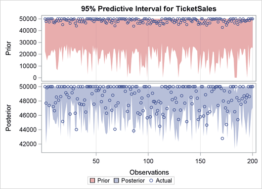
Output 22.8.2: Predictive Analysis by Observation Number
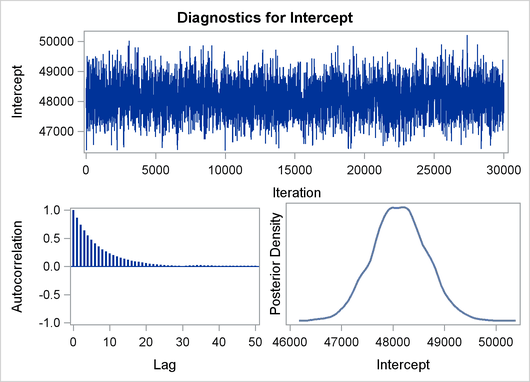
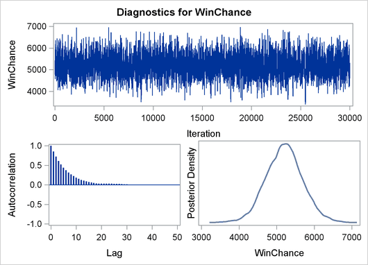
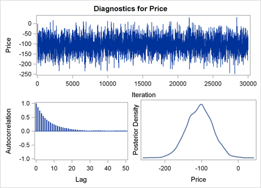
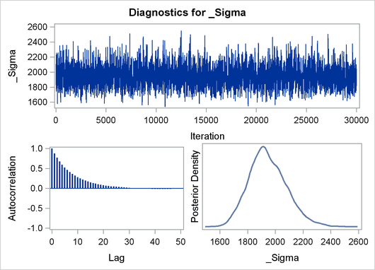
The validity of the MCMC sampling phase can be monitored with Output 22.8.3.
Output 22.8.3: Predictive Analysis by Observation Number
Finally the prior and the posterior predictive analyses are represented in Output 22.8.4
Output 22.8.4: Predictive Analysis by Observation Number