Alternate Distribution Simulation
As an alternate to the normal distribution, the ERRORMODEL statement can be used in a simulation to specify other distributions. The distributions available for simulation are Cauchy, chi-squared, F, Poisson, t, and uniform. An empirical distribution can also be used if the residuals are specified by using the RESIDDATA= option in the SOLVE statement.
Except for the t distribution, all of these alternate distributions are univariate but can be used together in a multivariate simulation. The ERRORMODEL statement applies to solved for equations only. That is, the normal form or general form equation referred to by the ERRORMODEL statement must be one of the equations you have selected in the SOLVE statement.
In the following example, two Poisson distributed variables are used to simulate the calls that arrive at and leave a call center.
data s;    /* Covariance between arriving and leaving */
   arriving = 1; leaving = 0.7; _name_= "arriving";
   output;
   arriving = 0.7; leaving = 1.0; _name_= "leaving";
   output;
run;

data calls;
   date = '20mar2001'd;
   output;
run;
The first DATA step generates a data set that contains a covariance matrix for the ARRIVING and LEAVING variables. The covariance is
|
|
The following statements create the number of waiting clients data:
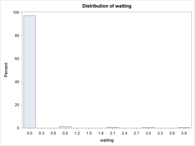
proc model data=calls;
   arriving = 0;
   errormodel arriving ~ poisson( 10 );
   leaving  = 4;
   errormodel leaving ~ poisson( 11 );

   waiting = arriving - leaving;
   if waiting < 0 then waiting=0;
   outvars waiting;

   solve arriving leaving / random=500 sdata=s out=sim;
run;

title "Distribution of Clients Waiting";
proc univariate data=sim noprint;
   var waiting ;
   histogram waiting / cfill=ligr;
run;
The distribution of number of waiting clients is shown in Figure 19.73.
Figure 19.73: Distribution of Number of Clients Waiting