The STATESPACE Procedure

The model is 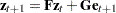, where is a sequence of independent multivariate normal innovations with mean vector 0 and variance . The observed sequence composes the first r components of , and thus , where H is the matrix .

Let be the matrix of innovations:

If the number of observations n is reasonably large, the log likelihood L can be approximated up to an additive constant as follows:

The elements of are taken as free parameters and are estimated as follows:

Replacing by in the likelihood equation, the log likelihood, up to an additive constant, is

Letting B be the backshift operator, the formal relation between and is

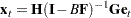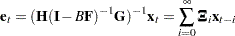Letting be the ith lagged sample covariance of and neglecting end effects, the matrix is

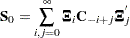For the computation of , the infinite sum is truncated at the value of the KLAG= option. The value of the KLAG= option should be large enough that the sequence is approximately 0 beyond that point.

Let be the vector of free parameters in the and matrices. The derivative of the log likelihood with respect to the parameter is

The second derivative is

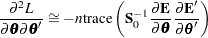
Near the maximum, the first term is unimportant and the second term can be approximated to give the following second derivative approximation:

The first derivative matrix and this second derivative matrix approximation are computed from the sample covariance matrix and the truncated sequence . The approximate likelihood function is maximized by a modified Newton-Raphson algorithm that employs these derivative matrices.

The matrix is used as the estimate of the innovation covariance matrix, . The negative of the inverse of the second derivative matrix at the maximum is used as an approximate covariance matrix for the parameter estimates. The standard errors of the parameter estimates printed in the parameter estimates tables are taken from the diagonal of this covariance matrix. The parameter covariance matrix is printed when the COVB option is specified.

If the data are nearly nonstationary, a better estimate of and the other parameters can sometimes be obtained by specifying the RESIDEST option. The RESIDEST option estimates the parameters by using conditional least squares instead of maximum likelihood.

The residuals are computed using the state space equation and the sample mean values of the variables in the model as start-up values. The estimate of is then computed using the residuals from the ith observation on, where i is the maximum number of times any variable occurs in the state vector. A multivariate Gauss-Marquardt algorithm is used to minimize . See Harvey (1981a) for a further description of this method.