| Nested Logit Modeling |
A more general model can be specified using the nested logit model.
Consider, for example, the following random utility function:
 |
Suppose the set of all alternatives indexed by  is partitioned into
  nests,
  . The nested logit model is obtained by assuming that the error term in the utility function has the GEV cumulative distribution function
 |
where  is a measure of a degree of independence among the alternatives in nest
  . When
  for all
  , the model reduces to the standard logit model.
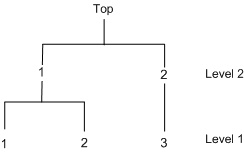
Since the public transportation modes, 1 and 2, tend to be correlated, these two choices can be grouped together. The decision tree displayed in Figure 18.8 is constructed.

The two-level decision tree is specified in the NEST statement. The NCHOICE= option is not allowed for nested logit estimation. Instead, the CHOICE= option needs to be specified, as in the following statements:
/*-- nested logit estimation --*/
proc mdc data=newdata;
   model decision = ttime /
            type=nlogit
            choice=(mode 1 2 3)
            covest=hess;
   id pid;
   utility u(1,) = ttime;
   nest level(1) = (1 2 @ 1, 3 @ 2),
        level(2) = (1 2 @ 1);
run;
In Figure 18.9, estimates of the inclusive value parameters, INC_L2G1C1 and INC_L2G1C2, are indicative of a nested model structure. See the section Nested Logit and the section Decision Tree and Nested Logit for more details about inclusive values.
| Parameter Estimates | |||||
|---|---|---|---|---|---|
| Parameter | DF | Estimate | Standard Error |
t Value | Approx Pr > |t| |
| ttime_L1 | 1 | -0.4040 | 0.1241 | -3.25 | 0.0011 |
| INC_L2G1C1 | 1 | 0.8016 | 0.4352 | 1.84 | 0.0655 |
| INC_L2G1C2 | 1 | 0.8087 | 0.3591 | 2.25 | 0.0243 |
The nested logit model is estimated with the restriction INC_L2G1C1 = INC_L2G1C2 by specifying the SAMESCALE option, as in the following statements:
/*-- nlogit with samescale option --*/
proc mdc data=newdata;
   model decision = ttime /
            type=nlogit
            choice=(mode 1 2 3)
            samescale
            covest=hess;
   id pid;
   utility u(1,) = ttime;
   nest level(1) = (1 2 @ 1, 3 @ 2),
        level(2) = (1 2 @ 1);
run;
The estimation result is displayed in Figure 18.10.
| Parameter Estimates | |||||
|---|---|---|---|---|---|
| Parameter | DF | Estimate | Standard Error |
t Value | Approx Pr > |t| |
| ttime_L1 | 1 | -0.4025 | 0.1217 | -3.31 | 0.0009 |
| INC_L2G1 | 1 | 0.8209 | 0.3019 | 2.72 | 0.0066 |
The nested logit model is equivalent to the conditional logit model if INC_L2G1C1 = INC_L2G1C2 =  . You can verify this relationship by estimating a constrained nested logit model as shown in the following statements. (See the section RESTRICT Statement for details about imposing linear restrictions on parameter estimates.)
/*-- constrained nested logit estimation --*/
proc mdc data=newdata;
   model decision = ttime /
            type=nlogit
            choice=(mode 1 2 3)
            covest=hess;
   id pid;
   utility u(1,) = ttime;
   nest level(1) = (1 2 @ 1, 3 @ 2),
        level(2) = (1 2 @ 1);
   restrict INC_L2G1C1 = 1, INC_L2G1C2 =1;
run;
The parameter estimates and the active linear constraints for the constrained nested logit model are displayed in Figure 18.11.
| Parameter Estimates | ||||||
|---|---|---|---|---|---|---|
| Parameter | DF | Estimate | Standard Error |
t Value | Approx Pr > |t| |
Parameter Label |
| ttime_L1 | 1 | -0.3572 | 0.0776 | -4.60 | <.0001 | |
| INC_L2G1C1 | 0 | 1.0000 | 0 | |||
| INC_L2G1C2 | 0 | 1.0000 | 0 | |||
| Restrict1 | 1 | -2.1706 | 8.4098 | -0.26 | 0.7993* | Linear EC [ 1 ] |
| Restrict2 | 1 | 3.6573 | 10.0001 | 0.37 | 0.7186* | Linear EC [ 2 ] |
| Linearly Independent Active Linear Constraints | |||||||
|---|---|---|---|---|---|---|---|
| 1 | 0 | = | -1.0000 | + | 1.0000 | * | INC_L2G1C1 |
| 2 | 0 | = | -1.0000 | + | 1.0000 | * | INC_L2G1C2 |