The FORECAST Procedure
- Overview
-
Getting Started
 Giving Dates to Forecast Values Computing Confidence Limits Form of the OUT= Data Set Plotting Forecasts Plotting Residuals Model Parameters and Goodness-of-Fit Statistics Controlling the Forecasting Method Introduction to Forecasting Methods Time Trend Models Time Series Methods Combining Time Trend with Autoregressive Models
 -
Syntax
-
Details
-
Examples
- References
Example 16.1 Forecasting Auto Sales
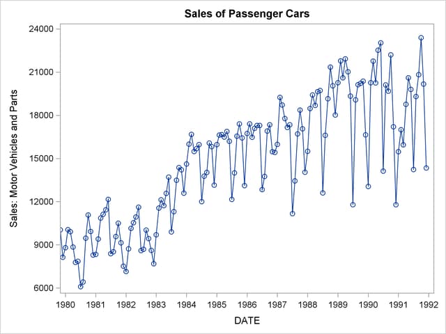
This example uses the Winters method to forecast the monthly U. S. sales of passenger cars series (VEHICLES) from the data set SASHELP.USECON. These data are taken from Business Statistics, published by the U. S. Bureau of Economic Analysis.
The following statements plot the series. The plot is shown in Output 16.1.1.
title1 "Sales of Passenger Cars";

symbol1 i=spline v=dot;
axis2 label=(a=-90 r=90 "Vehicles and Parts" )
      order=(6000 to 24000 by 3000);

title1 "Sales of Passenger Cars";
proc sgplot data=sashelp.usecon;
   series x=date y=vehicles / markers;
   xaxis values=('1jan80'd to '1jan92'd by year);
   yaxis values=(6000 to 24000 by 3000);
   format date year4.;
run;
The following statements produce the forecast:
proc forecast data=sashelp.usecon interval=month
              method=winters seasons=month lead=12
              out=out outfull outresid outest=est;
   id date;
   var vehicles;
   where date >= '1jan80'd;
run;
The INTERVAL=MONTH option indicates that the data are monthly, and the ID DATE statement gives the dating variable. The METHOD=WINTERS specifies the Winters smoothing method. The LEAD=12 option forecasts 12 months ahead. The OUT=OUT option specifies the output data set, while the OUTFULL and OUTRESID options include in the OUT= data set the predicted and residual values for the historical period and the confidence limits for the forecast period. The OUTEST= option stores various statistics in an output data set. The WHERE statement is used to include only data from 1980 on.
The following statements print the OUT= data set (first 20 observations):
title2 'The OUT= Data Set';
proc print data=out (obs=20) noobs;
run;
The listing of the output data set produced by PROC PRINT is shown in part in Output 16.1.2.
| Sales of Passenger Cars |
| The OUT= Data Set |
| DATE | _TYPE_ | _LEAD_ | VEHICLES |
|---|---|---|---|
| JAN80 | ACTUAL | 0 | 8808.00 |
| JAN80 | FORECAST | 0 | 8046.52 |
| JAN80 | RESIDUAL | 0 | 761.48 |
| FEB80 | ACTUAL | 0 | 10054.00 |
| FEB80 | FORECAST | 0 | 9284.31 |
| FEB80 | RESIDUAL | 0 | 769.69 |
| MAR80 | ACTUAL | 0 | 9921.00 |
| MAR80 | FORECAST | 0 | 10077.33 |
| MAR80 | RESIDUAL | 0 | -156.33 |
| APR80 | ACTUAL | 0 | 8850.00 |
| APR80 | FORECAST | 0 | 9737.21 |
| APR80 | RESIDUAL | 0 | -887.21 |
| MAY80 | ACTUAL | 0 | 7780.00 |
| MAY80 | FORECAST | 0 | 9335.24 |
| MAY80 | RESIDUAL | 0 | -1555.24 |
| JUN80 | ACTUAL | 0 | 7856.00 |
| JUN80 | FORECAST | 0 | 9597.50 |
| JUN80 | RESIDUAL | 0 | -1741.50 |
| JUL80 | ACTUAL | 0 | 6102.00 |
| JUL80 | FORECAST | 0 | 6833.16 |
The following statements print the OUTEST= data set:
title2 'The OUTEST= Data Set: WINTERS Method';
proc print data=est;
run;
The PROC PRINT listing of the OUTEST= data set is shown in Output 16.1.3.
| Sales of Passenger Cars |
| The OUTEST= Data Set: WINTERS Method |
| Obs | _TYPE_ | DATE | VEHICLES |
|---|---|---|---|
| 1 | N | DEC91 | 144 |
| 2 | NRESID | DEC91 | 144 |
| 3 | DF | DEC91 | 130 |
| 4 | WEIGHT1 | DEC91 | 0.1055728 |
| 5 | WEIGHT2 | DEC91 | 0.1055728 |
| 6 | WEIGHT3 | DEC91 | 0.25 |
| 7 | SIGMA | DEC91 | 1741.481 |
| 8 | CONSTANT | DEC91 | 18577.368 |
| 9 | LINEAR | DEC91 | 4.804732 |
| 10 | S_JAN | DEC91 | 0.8909173 |
| 11 | S_FEB | DEC91 | 1.0500278 |
| 12 | S_MAR | DEC91 | 1.0546539 |
| 13 | S_APR | DEC91 | 1.074955 |
| 14 | S_MAY | DEC91 | 1.1166121 |
| 15 | S_JUN | DEC91 | 1.1012972 |
| 16 | S_JUL | DEC91 | 0.7418297 |
| 17 | S_AUG | DEC91 | 0.9633888 |
| 18 | S_SEP | DEC91 | 1.051159 |
| 19 | S_OCT | DEC91 | 1.1399126 |
| 20 | S_NOV | DEC91 | 1.0132126 |
| 21 | S_DEC | DEC91 | 0.802034 |
| 22 | SST | DEC91 | 2.63312E9 |
| 23 | SSE | DEC91 | 394258270 |
| 24 | MSE | DEC91 | 3032755.9 |
| 25 | RMSE | DEC91 | 1741.481 |
| 26 | MAPE | DEC91 | 9.4800217 |
| 27 | MPE | DEC91 | -1.049956 |
| 28 | MAE | DEC91 | 1306.8534 |
| 29 | ME | DEC91 | -42.95376 |
| 30 | RSQUARE | DEC91 | 0.8502696 |
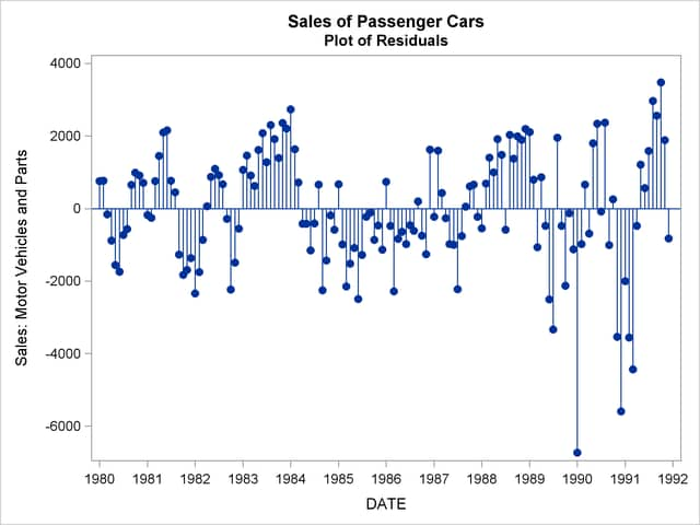
The following statements plot the residuals. The plot is shown in Output 16.1.4.
title1 "Sales of Passenger Cars";
title2 'Plot of Residuals';
proc sgplot data=out;
   where _type_ = 'RESIDUAL';
   needle x=date y=vehicles / markers markerattrs=(symbol=circlefilled);
   xaxis values=('1jan80'd to '1jan92'd by year);
   format date year4.;
run;
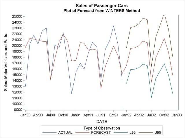
The following statements plot the forecast and confidence limits. The last two years of historical data are included in the plot to provide context for the forecast plot. A reference line is drawn at the start of the forecast period.
title1 "Sales of Passenger Cars";
title2 'Plot of Forecast from WINTERS Method';
proc sgplot data=out;
   series x=date y=vehicles / group=_type_ lineattrs=(pattern=1);
   where _type_ ^= 'RESIDUAL';
   refline '15dec91'd / axis=x;
   yaxis values=(9000 to 25000 by 1000);
   xaxis values=('1jan90'd to '1jan93'd by qtr);
run;
The plot is shown in Output 16.1.5.