| The VARMAX Procedure |
| Vector Error Correction Modeling |
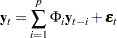
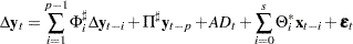
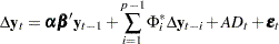
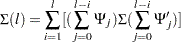
This section discusses the implication of cointegration for the autoregressive representation. Assume that the cointegrated series can be represented by a vector error correction model according to the Granger representation theorem (Engle and Granger 1987). Consider the vector autoregressive process with Gaussian errors defined by
 |
or
 |
where the initial values,  , are fixed and
  . Since the AR operator
  can be re-expressed as
  , where
 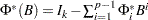 with
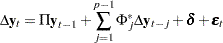
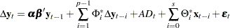
with 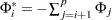 , the vector error correction model is
 |
or
 |
where  .
.
One motivation for the VECM( ) form is to consider the relation
  as defining the underlying economic relations and assume that the agents react to the disequilibrium error
  through the adjustment coefficient
  to restore equilibrium; that is, they satisfy the economic relations. The cointegrating vector,
  is sometimes called the long-run parameters.
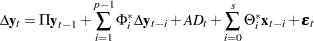
You can consider a vector error correction model with a deterministic term. The deterministic term  can contain a constant, a linear trend, and seasonal dummy variables. Exogenous variables can also be included in the model.
 |
where  .
.
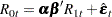
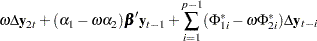
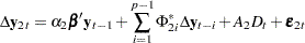
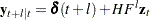
The alternative vector error correction representation considers the error correction term at lag  and is written as
 |
If the matrix  has a full-rank (
 ), all components of
  are
are  . On the other hand, are stationary in difference if
  . When the rank of the matrix is
  , there are
  linear combinations that are nonstationary and
  stationary cointegrating relations. Note that the linearly independent vector
  is stationary and this transformation is not unique unless
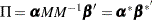
  . There does not exist a unique cointegrating matrix since the coefficient matrix can also be decomposed as
 |
where  is an
is an  nonsingular matrix.
Test for the Cointegration
The cointegration rank test determines the linearly independent columns of . Johansen (1988, 1995a) and Johansen and Juselius (1990) proposed the cointegration rank test by using the reduced rank regression.
When you construct the VECM() form from the VAR() model, the deterministic terms in the VECM() form can differ from those in the VAR() model. When there are deterministic cointegrated relationships among variables, deterministic terms in the VAR() model are not present in the VECM() form. On the other hand, if there are stochastic cointegrated relationships in the VAR() model, deterministic terms appear in the VECM() form via the error correction term or as an independent term in the VECM() form. There are five different specifications of deterministic trends in the VECM() form.
Case 1: There is no separate drift in the VECM(
) form. 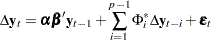
Case 2: There is no separate drift in the VECM(
) form, but a constant enters only via the error correction term. 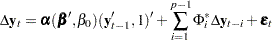
Case 3: There is a separate drift and no separate linear trend in the VECM(
) form. 
Case 4: There is a separate drift and no separate linear trend in the VECM(
) form, but a linear trend enters only via the error correction term. 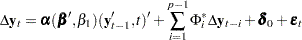
Case 5: There is a separate linear trend in the VECM(
) form. 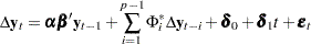
First, focus on Cases 1, 3, and 5 to test the null hypothesis that there are at most cointegrating vectors. Let
 |
 |
 |
|||
 |
|
 |
|||
 |
|
 |
|||
 |
|
 |
|||
 |
|
 |
|||
 |
|
 |
where can be empty for Case 1, 1 for Case 3, and  for Case 5.
In Case 2,  and
and  are defined as
 |
|
 |
|||
|
|
 |
In Case 4, and are defined as
|
|
 |
|||
|
|
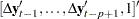 |
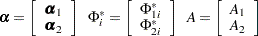
Let  be the matrix of parameters consisting of
  , ...,
  ,
,  , and
, and  , ...,
  , where parameters corresponds to regressors . Then the VECM() form is rewritten in these variables as
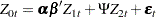 |
The log-likelihood function is given by
 |
|
 |
|||
 |
|
 |
The residuals,  and
and  , are obtained by regressing
  and on , respectively. The regression equation of residuals is
 |
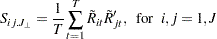
The crossproducts matrices are computed
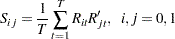 |
Then the maximum likelihood estimator for is obtained from the eigenvectors that correspond to the largest eigenvalues of the following equation:
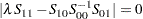 |
The eigenvalues of the preceding equation are squared canonical correlations between and , and the eigenvectors that correspond to the largest eigenvalues are the linear combinations of  , which have the largest squared partial correlations with the stationary process
  after correcting for lags and deterministic terms. Such an analysis calls for a reduced rank regression of on corrected for
  , as discussed by Anderson (1951). Johansen (1988) suggests two test statistics to test the null hypothesis that there are at most cointegrating vectors
 |
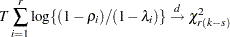
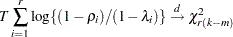
The trace statistic for testing the null hypothesis that there are at most cointegrating vectors is as follows:
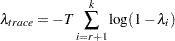 |
The asymptotic distribution of this statistic is given by
 |
where  is the trace of a matrix ,
  is the dimensional Brownian motion, and
  is the Brownian motion itself, or the demeaned or detrended Brownian motion according to the different specifications of deterministic trends in the vector error correction model.
The maximum eigenvalue statistic for testing the null hypothesis that there are at most cointegrating vectors is as follows:
 |
The asymptotic distribution of this statistic is given by
 |
where  is the maximum eigenvalue of a matrix . Osterwald-Lenum (1992) provided detailed tables of the critical values of these statistics.
The following statements use the JOHANSEN option to compute the Johansen cointegration rank trace test of integrated order 1:
proc varmax data=simul2;
   model y1 y2 / p=2 cointtest=(johansen=(normalize=y1));
run;
Figure 32.52 shows the output based on the model specified in the MODEL statement, an intercept term is assumed. In the "Cointegration Rank Test Using Trace" table, the column Drift In ECM means there is no separate drift in the error correction model and the column Drift In Process means the process has a constant drift before differencing. The "Cointegration Rank Test Using Trace" table shows the trace statistics based on Case 3 and the "Cointegration Rank Test Using Trace under Restriction" table shows the trace statistics based on Case 2. The output indicates that the series are cointegrated with rank 1 because the trace statistics are smaller than the critical values in both Case 2 and Case 3.
| Cointegration Rank Test Using Trace | ||||||
|---|---|---|---|---|---|---|
| H0: Rank=r |
H1: Rank>r |
Eigenvalue | Trace | 5% Critical Value | Drift in ECM | Drift in Process |
| 0 | 0 | 0.4644 | 61.7522 | 15.34 | Constant | Linear |
| 1 | 1 | 0.0056 | 0.5552 | 3.84 | ||
| Cointegration Rank Test Using Trace Under Restriction | ||||||
|---|---|---|---|---|---|---|
| H0: Rank=r |
H1: Rank>r |
Eigenvalue | Trace | 5% Critical Value | Drift in ECM | Drift in Process |
| 0 | 0 | 0.5209 | 76.3788 | 19.99 | Constant | Constant |
| 1 | 1 | 0.0426 | 4.2680 | 9.13 | ||
Figure 32.53 shows which result, either Case 2 (the hypothesis H0) or Case 3 (the hypothesis H1), is appropriate depending on the significance level. Since the cointegration rank is chosen to be 1 by the result in Figure 32.52, look at the last row that corresponds to rank=1. Since the -value is 0.054, the Case 2 cannot be rejected at the significance level 5%, but it can be rejected at the significance level 10%. For modeling of the two Case 2 and Case 3, see Figure 32.56 and Figure 32.57.
Figure 32.54 shows the estimates of long-run parameter (Beta) and adjustment coefficients (Alpha) based on Case 3.
Using the NORMALIZE= option, the first low of the "Beta" table has 1. Considering that the cointegration rank is 1, the long-run relationship of the series is
 |
|
 |
|||
|
|
 |
|||
 |
|
 |
Figure 32.55 shows the estimates of long-run parameter (Beta) and adjustment coefficients (Alpha) based on Case 2.
Considering that the cointegration rank is 1, the long-run relationship of the series is
|
|
 |
|||
|
|
 |
|||
|
|
 |
Estimation of Vector Error Correction Model
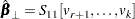
The preceding log-likelihood function is maximized for
 |
|
 |
|||
 |
|
 |
|||
 |
|
 |
|||
 |
|
 |
|||
 |
|
 |
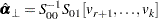
The estimators of the orthogonal complements of and are
 |
and
 |
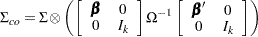
The ML estimators have the following asymptotic properties:
 |
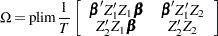
where
 |
and
 |
The following statements are examples of fitting the five different cases of the vector error correction models mentioned in the previous section.
For fitting Case 1,
model y1 y2 / p=2 ecm=(rank=1 normalize=y1) noint;
For fitting Case 2,
model y1 y2 / p=2 ecm=(rank=1 normalize=y1 ectrend);
For fitting Case 3,
model y1 y2 / p=2 ecm=(rank=1 normalize=y1);
   model y1 y2 / p=2 ecm=(rank=1 normalize=y1 ectrend)
                 trend=linear;
For fitting Case 5,
model y1 y2 / p=2 ecm=(rank=1 normalize=y1) trend=linear;
From Figure 32.53 that uses the COINTTEST=(JOHANSEN) option, you can fit the model by using either Case 2 or Case 3 because the test was not significant at the 0.05 level, but was significant at the 0.10 level. Here both models are fitted to show the difference in output display. Figure 32.56 is for Case 2, and Figure 32.57 is for Case 3.
For Case 2,
proc varmax data=simul2;
   model y1 y2 / p=2 ecm=(rank=1 normalize=y1 ectrend)
                 print=(estimates);
run;
| Parameter Alpha * Beta' Estimates | |||
|---|---|---|---|
| Variable | y1 | y2 | 1 |
| y1 | -0.48015 | 0.98126 | -3.24543 |
| y2 | 0.12538 | -0.25624 | 0.84748 |
| AR Coefficients of Differenced Lag | |||
|---|---|---|---|
| DIF Lag | Variable | y1 | y2 |
| 1 | y1 | -0.72759 | -0.77463 |
| y2 | 0.38982 | -0.55173 | |
| Model Parameter Estimates | ||||||
|---|---|---|---|---|---|---|
| Equation | Parameter | Estimate | Standard Error |
t Value | Pr > |t| | Variable |
| D_y1 | CONST1 | -3.24543 | 0.33022 | 1, EC | ||
| AR1_1_1 | -0.48015 | 0.04886 | y1(t-1) | |||
| AR1_1_2 | 0.98126 | 0.09984 | y2(t-1) | |||
| AR2_1_1 | -0.72759 | 0.04623 | -15.74 | 0.0001 | D_y1(t-1) | |
| AR2_1_2 | -0.77463 | 0.04978 | -15.56 | 0.0001 | D_y2(t-1) | |
| D_y2 | CONST2 | 0.84748 | 0.35394 | 1, EC | ||
| AR1_2_1 | 0.12538 | 0.05236 | y1(t-1) | |||
| AR1_2_2 | -0.25624 | 0.10702 | y2(t-1) | |||
| AR2_2_1 | 0.38982 | 0.04955 | 7.87 | 0.0001 | D_y1(t-1) | |
| AR2_2_2 | -0.55173 | 0.05336 | -10.34 | 0.0001 | D_y2(t-1) | |
Figure 32.56 can be reported as follows:
 |
|
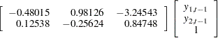 |
|||
|
|
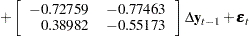 |
The keyword "EC" in the "Model Parameter Estimates" table means that the ECTREND option is used for fitting the model.
For fitting Case 3,
proc varmax data=simul2;
   model y1 y2 / p=2 ecm=(rank=1 normalize=y1)
                 print=(estimates);
run;
| Parameter Alpha * Beta' Estimates | ||
|---|---|---|
| Variable | y1 | y2 |
| y1 | -0.46421 | 0.95103 |
| y2 | 0.17535 | -0.35923 |
| AR Coefficients of Differenced Lag | |||
|---|---|---|---|
| DIF Lag | Variable | y1 | y2 |
| 1 | y1 | -0.74052 | -0.76305 |
| y2 | 0.34820 | -0.51194 | |
| Model Parameter Estimates | ||||||
|---|---|---|---|---|---|---|
| Equation | Parameter | Estimate | Standard Error |
t Value | Pr > |t| | Variable |
| D_y1 | CONST1 | -2.60825 | 1.32398 | -1.97 | 0.0518 | 1 |
| AR1_1_1 | -0.46421 | 0.05474 | y1(t-1) | |||
| AR1_1_2 | 0.95103 | 0.11215 | y2(t-1) | |||
| AR2_1_1 | -0.74052 | 0.05060 | -14.63 | 0.0001 | D_y1(t-1) | |
| AR2_1_2 | -0.76305 | 0.05352 | -14.26 | 0.0001 | D_y2(t-1) | |
| D_y2 | CONST2 | 3.43005 | 1.39587 | 2.46 | 0.0159 | 1 |
| AR1_2_1 | 0.17535 | 0.05771 | y1(t-1) | |||
| AR1_2_2 | -0.35923 | 0.11824 | y2(t-1) | |||
| AR2_2_1 | 0.34820 | 0.05335 | 6.53 | 0.0001 | D_y1(t-1) | |
| AR2_2_2 | -0.51194 | 0.05643 | -9.07 | 0.0001 | D_y2(t-1) | |
Figure 32.57 can be reported as follows:
|
|
 |
|||
|
|
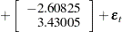 |
Test for the Linear Restriction on the Parameters
Consider the example with the variables  log real money,
  log real income,
  deposit interest rate, and
  bond interest rate. It seems a natural hypothesis that in the long-run relation, money and income have equal coefficients with opposite signs. This can be formulated as the hypothesis that the cointegrated relation contains only and through
  . For the analysis, you can express these restrictions in the parameterization of
  such that
  , where is a known
  matrix and
  is the
  parameter matrix to be estimated. For this example, is given by
 |

When the linear restriction is given, it implies that the same restrictions are imposed on all cointegrating vectors. You obtain the maximum likelihood estimator of by reduced rank regression of  on
on  corrected for
  , solving the following equation
 |
for the eigenvalues 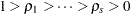 and eigenvectors
  ,
,  given in the preceding section. Then choose
  that corresponds to the largest eigenvalues, and the
  is
is  .
.
The test statistic for is given by
 |
If the series has no deterministic trend, the constant term should be restricted by  as in Case 2. Then is given by
 |
The following statements test that 2  :
:
proc varmax data=simul2;
   model y1 y2 / p=2 ecm=(rank=1 normalize=y1);
   cointeg rank=1 h=(1,-2);
run;
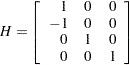
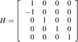
Figure 32.58 shows the results of testing 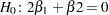 . The input matrix is
  . The adjustment coefficient is reestimated under the restriction, and the test indicates that you cannot reject the null hypothesis.
| Beta Under Restriction | |
|---|---|
| Variable | 1 |
| y1 | 1.00000 |
| y2 | -2.00000 |
| Alpha Under Restriction | |
|---|---|
| Variable | 1 |
| y1 | -0.47404 |
| y2 | 0.17534 |
| Hypothesis Test | |||||
|---|---|---|---|---|---|
| Index | Eigenvalue | Restricted Eigenvalue |
DF | Chi-Square | Pr > ChiSq |
| 1 | 0.4644 | 0.4616 | 1 | 0.51 | 0.4738 |
Test for the Weak Exogeneity and Restrictions of Alpha
Consider a vector error correction model:
 |
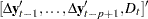
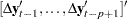
Divide the process into  with dimension
  and
and  and the
  into
into
 |
Similarly, the parameters can be decomposed as follows:
 |
Then the VECM(p) form can be rewritten by using the decomposed parameters and processes:
 |
The conditional model for  given
given  is
is
 |
|
 |
|||
|
|
 |
and the marginal model of is
 |
where  .
.
The test of weak exogeneity of for the parameters  determines whether
  . Weak exogeneity means that there is no information about in the marginal model or that the variables do not react to a disequilibrium.

Consider the null hypothesis  , where
  is a
is a  matrix with
  .
.
From the previous residual regression equation
 |
you can obtain
 |
|
 |
|||
 |
|
 |
where  and
and  is orthogonal to such that
  .
.
Define
 |
and let  . Then
  can be written as
 |
Using the marginal distribution of  and the conditional distribution of , the new residuals are computed as
 |
 |
 |
|||
 |
|
 |
where
 |
In terms of  and
and  , the MLE of is computed by using the reduced rank regression. Let
 |
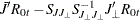
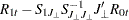
Under the null hypothesis , the MLE  is computed by solving the equation
 |
Then  , where the eigenvectors correspond to the largest eigenvalues. The likelihood ratio test for is
 |
The test of weak exogeneity of is a special case of the test  , considering
  . Consider the previous example with four variables (
  ). If , you formulate the weak exogeneity of (
 ) for as
  and the weak exogeneity of
  for (
for ( ) as
) as  .
.
The following statements test the weak exogeneity of other variables, assuming :
proc varmax data=simul2;
   model y1 y2 / p=2 ecm=(rank=1 normalize=y1);
   cointeg rank=1 exogeneity;
run;
proc varmax data=simul2;
   model y1 y2 / p=2 ecm=(rank=1 normalize=y1);
   cointeg rank=1 j=exogeneity;
run;
Figure 32.59 shows that each variable is not the weak exogeneity of other variable.
| Testing Weak Exogeneity of Each Variables |
|||
|---|---|---|---|
| Variable | DF | Chi-Square | Pr > ChiSq |
| y1 | 1 | 53.46 | <.0001 |
| y2 | 1 | 8.76 | 0.0031 |
Forecasting of the VECM
Consider the cointegrated moving-average representation of the differenced process of 
 |
Assume that  . The linear process can be written as
 |
Therefore, for any  ,
,
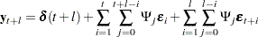 |
The  -step-ahead forecast is derived from the preceding equation:
 |
Note that
 |
since 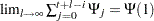 and
and  . The long-run forecast of the cointegrated system shows that the cointegrated relationship holds, although there might exist some deviations from the equilibrium status in the short-run. The covariance matrix of the predict error
  is
is
 |
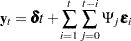
When the linear process is represented as a VECM() model, you can obtain
 |
The transition equation is defined as
 |
where  is a state vector and the transition matrix is
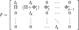 |
where 0 is a  zero matrix. The observation equation can be written
 |
where 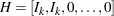 .
.
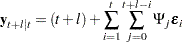
The -step-ahead forecast is computed as
 |
Cointegration with Exogenous Variables
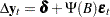
The error correction model with exogenous variables can be written as follows:
 |
The following statements demonstrate how to fit VECMX( ), where
  and
and  from the P=2 and XLAG=1 options:
   proc varmax data=simul3;
      model y1 y2 = x1 / p=2 xlag=1 ecm=(rank=1);
   run;
The following statements demonstrate how to BVECMX(2,1):
   proc varmax data=simul3;
      model y1 y2 = x1 / p=2 xlag=1 ecm=(rank=1)
         prior=(lambda=0.9 theta=0.1);
   run;
Copyright © SAS Institute, Inc. All Rights Reserved.