| The VARMAX Procedure |
| Vector Autoregressive Process with Exogenous Variables |
A VAR process can be affected by other observable variables that are determined outside the system of interest. Such variables are called exogenous (independent) variables. Exogenous variables can be stochastic or nonstochastic. The process can also be affected by the lags of exogenous variables. A model used to describe this process is called a VARX( ,
, ) model.
The VARX(,) model is written as
 |
where  is an
is an  -dimensional time series vector and
  is a
is a  matrix.
For example, a VARX(1,0) model is
 |
where  and
and  .
.
The following statements fit the VARX(1,0) model to the given data:
data grunfeld;
   input year y1 y2 y3 x1 x2 x3;
   label y1='Gross Investment GE'
         y2='Capital Stock Lagged GE'
         y3='Value of Outstanding Shares GE Lagged'
         x1='Gross Investment W'
         x2='Capital Stock Lagged W'
         x3='Value of Outstanding Shares Lagged W';
datalines;
1935  33.1 1170.6  97.8 12.93  191.5   1.8
1936  45.0 2015.8 104.4 25.90  516.0    .8
1937  77.2 2803.3 118.0 35.05  729.0   7.4

   ... more lines ...
/*--- Vector Autoregressive Process with Exogenous Variables ---*/

proc varmax data=grunfeld;
   model y1-y3 = x1 x2 / p=1 lagmax=5
                         printform=univariate
                         print=(impulsx=(all) estimates);
run;
The VARMAX procedure output is shown in Figure 32.18 through Figure 32.20.
Figure 32.18 shows the descriptive statistics for the dependent (endogenous) and independent (exogenous) variables with labels.
| Number of Observations | 20 |
|---|---|
| Number of Pairwise Missing | 0 |
| Simple Summary Statistics | |||||||
|---|---|---|---|---|---|---|---|
| Variable | Type | N | Mean | Standard Deviation |
Min | Max | Label |
| y1 | Dependent | 20 | 102.29000 | 48.58450 | 33.10000 | 189.60000 | Gross Investment GE |
| y2 | Dependent | 20 | 1941.32500 | 413.84329 | 1170.60000 | 2803.30000 | Capital Stock Lagged GE |
| y3 | Dependent | 20 | 400.16000 | 250.61885 | 97.80000 | 888.90000 | Value of Outstanding Shares GE Lagged |
| x1 | Independent | 20 | 42.89150 | 19.11019 | 12.93000 | 90.08000 | Gross Investment W |
| x2 | Independent | 20 | 670.91000 | 222.39193 | 191.50000 | 1193.50000 | Capital Stock Lagged W |
Figure 32.19 shows the parameter estimates for the constant, the lag zero coefficients of exogenous variables, and the lag one AR coefficients. From the schematic representation of parameter estimates, the significance of the parameter estimates can be easily verified. The symbol "C" means the constant and "XL0" means the lag zero coefficients of exogenous variables.
| Type of Model | VARX(1,0) |
|---|---|
| Estimation Method | Least Squares Estimation |
| Constant | |
|---|---|
| Variable | Constant |
| y1 | -12.01279 |
| y2 | 702.08673 |
| y3 | -22.42110 |
| XLag | |||
|---|---|---|---|
| Lag | Variable | x1 | x2 |
| 0 | y1 | 1.69281 | -0.00859 |
| y2 | -6.09850 | 2.57980 | |
| y3 | -0.02317 | -0.01274 | |
| AR | ||||
|---|---|---|---|---|
| Lag | Variable | y1 | y2 | y3 |
| 1 | y1 | 0.23699 | 0.00763 | 0.02941 |
| y2 | -2.46656 | 0.16379 | -0.84090 | |
| y3 | 0.95116 | 0.00224 | 0.93801 | |
| Schematic Representation | |||
|---|---|---|---|
| Variable/Lag | C | XL0 | AR1 |
| y1 | . | +. | ... |
| y2 | + | .+ | ... |
| y3 | - | .. | +.+ |
| + is > 2*std error, - is < -2*std error, . is between, * is N/A | |||
Figure 32.20 shows the parameter estimates and their significance.
| Model Parameter Estimates | ||||||
|---|---|---|---|---|---|---|
| Equation | Parameter | Estimate | Standard Error |
t Value | Pr > |t| | Variable |
| y1 | CONST1 | -12.01279 | 27.47108 | -0.44 | 0.6691 | 1 |
| XL0_1_1 | 1.69281 | 0.54395 | 3.11 | 0.0083 | x1(t) | |
| XL0_1_2 | -0.00859 | 0.05361 | -0.16 | 0.8752 | x2(t) | |
| AR1_1_1 | 0.23699 | 0.20668 | 1.15 | 0.2722 | y1(t-1) | |
| AR1_1_2 | 0.00763 | 0.01627 | 0.47 | 0.6470 | y2(t-1) | |
| AR1_1_3 | 0.02941 | 0.04852 | 0.61 | 0.5548 | y3(t-1) | |
| y2 | CONST2 | 702.08673 | 256.48046 | 2.74 | 0.0169 | 1 |
| XL0_2_1 | -6.09850 | 5.07849 | -1.20 | 0.2512 | x1(t) | |
| XL0_2_2 | 2.57980 | 0.50056 | 5.15 | 0.0002 | x2(t) | |
| AR1_2_1 | -2.46656 | 1.92967 | -1.28 | 0.2235 | y1(t-1) | |
| AR1_2_2 | 0.16379 | 0.15193 | 1.08 | 0.3006 | y2(t-1) | |
| AR1_2_3 | -0.84090 | 0.45304 | -1.86 | 0.0862 | y3(t-1) | |
| y3 | CONST3 | -22.42110 | 10.31166 | -2.17 | 0.0487 | 1 |
| XL0_3_1 | -0.02317 | 0.20418 | -0.11 | 0.9114 | x1(t) | |
| XL0_3_2 | -0.01274 | 0.02012 | -0.63 | 0.5377 | x2(t) | |
| AR1_3_1 | 0.95116 | 0.07758 | 12.26 | 0.0001 | y1(t-1) | |
| AR1_3_2 | 0.00224 | 0.00611 | 0.37 | 0.7201 | y2(t-1) | |
| AR1_3_3 | 0.93801 | 0.01821 | 51.50 | 0.0001 | y3(t-1) | |
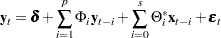
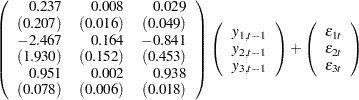
The fitted model is given as
 |
 |
 |
|||
 |
 |
 |
Copyright © SAS Institute, Inc. All Rights Reserved.