| The VARMAX Procedure |
| Vector Error Correction Model |
A vector error correction model (VECM) can lead to a better understanding of the nature of any nonstationarity among the different component series and can also improve longer term forecasting over an unconstrained model.
The VECM( ) form with the cointegration rank
  is written as
 |
where  is the differencing operator, such that
  ;
;  , where
  and
and  are
are  matrices;
  is a
is a  matrix.
It has an equivalent VAR() representation as described in the preceding section.
 |
where  is a identity matrix.
Example of Vector Error Correction Model
An example of the second-order nonstationary vector autoregressive model is
 |
with
 |
This process can be given the following VECM(2) representation with the cointegration rank one:
 |
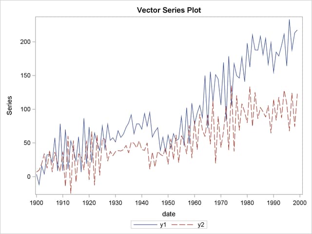
The following PROC IML statements generate simulated data for the VECM(2) form specified above and plot the data as shown in Figure 32.12:
proc iml;
   sig = 100*i(2);
   phi = {-0.2 0.1, 0.5 0.2, 0.8 0.7, -0.4 0.6};
   call varmasim(y,phi) sigma=sig n=100 initial=0
                        seed=45876;
   cn = {'y1' 'y2'};
   create simul2 from y[colname=cn];
   append from y;
quit;

data simul2;
   set simul2;
   date = intnx( 'year', '01jan1900'd, _n_-1 );
   format date year4. ;
run;
proc timeseries data=simul2 vectorplot=series;
   id date interval=year;
   var y1 y2;
run;
Cointegration Testing
The following statements use the Johansen cointegration rank test. The COINTTEST=(JOHANSEN) option does the Johansen trace test and is equivalent to specifying COINTTEST with no additional options or the COINTTEST=(JOHANSEN=(TYPE=TRACE)) option.
/*--- Cointegration Test ---*/

proc varmax data=simul2;
   model y1 y2 / p=2 noint dftest cointtest=(johansen);
run;
Figure 32.13 shows the output for Dickey-Fuller tests for the nonstationarity of each series and Johansen cointegration rank test between series.
| Unit Root Test | |||||
|---|---|---|---|---|---|
| Variable | Type | Rho | Pr < Rho | Tau | Pr < Tau |
| y1 | Zero Mean | 1.47 | 0.9628 | 1.65 | 0.9755 |
| Single Mean | -0.80 | 0.9016 | -0.47 | 0.8916 | |
| Trend | -10.88 | 0.3573 | -2.20 | 0.4815 | |
| y2 | Zero Mean | -0.05 | 0.6692 | -0.03 | 0.6707 |
| Single Mean | -6.03 | 0.3358 | -1.72 | 0.4204 | |
| Trend | -50.49 | 0.0003 | -4.92 | 0.0006 | |
| Cointegration Rank Test Using Trace | ||||||
|---|---|---|---|---|---|---|
| H0: Rank=r |
H1: Rank>r |
Eigenvalue | Trace | 5% Critical Value | Drift in ECM | Drift in Process |
| 0 | 0 | 0.5086 | 70.7279 | 12.21 | NOINT | Constant |
| 1 | 1 | 0.0111 | 1.0921 | 4.14 | ||
In Dickey-Fuller tests, the second column specifies three types of models, which are zero mean, single mean, or trend. The third column ( Rho ) and the fifth column ( Tau ) are the test statistics for unit root testing. Other columns are their -values. You can see that both series have unit roots. For a description of Dickey-Fuller tests, see the section PROBDF Function for Dickey-Fuller Tests in
Chapter 5,
SAS Macros and Functions.
In the cointegration rank test, the last two columns explain the drift in the model or process. Since the NOINT option is specified, the model is
 |
The column Drift In ECM means there is no separate drift in the error correction model, and the column Drift In Process means the process has a constant drift before differencing.
H0 is the null hypothesis, and H1 is the alternative hypothesis. The first row tests  against
  ; the second row tests
  against
  . The Trace test statistics in the fourth column are computed by
  where
where  is the available number of observations and
  is the eigenvalue in the third column. By default, the critical values at 5% significance level are used for testing. You can compare the test statistics and critical values in each row. There is one cointegrated process in this example since the Trace statistic for testing against is greater than the critical value, but the Trace statistic for testing against is not greater than the critical value.
The following statements fit a VECM(2) form to the simulated data. From the result in Figure 32.13, the time series are cointegrated with rank=1. You specify the ECM= option with the RANK=1 option. For normalizing the value of the cointegrated vector, you specify the normalized variable with the NORMALIZE= option. The PRINT=(IARR) option provides the VAR(2) representation. The VARMAX procedure output is shown in Figure 32.14 through Figure 32.16.
/*--- Vector Error-Correction Model ---*/

proc varmax data=simul2;
   model y1 y2 / p=2 noint lagmax=3
                 ecm=(rank=1 normalize=y1)
                 print=(iarr estimates);
run;
The ECM= option produces the estimates of the long-run parameter,  , and the adjustment coefficient,
  . In Figure 32.14, "1" indicates the first column of the and matrices. Since the cointegration rank is 1 in the bivariate system, and are two-dimensional vectors. The estimated cointegrating vector is
  . Therefore, the long-run relationship between
  and
and  is
is  . The first element of
  is 1 since
  is specified as the normalized variable.
| Type of Model | VECM(2) |
|---|---|
| Estimation Method | Maximum Likelihood Estimation |
| Cointegrated Rank | 1 |
| Beta | |
|---|---|
| Variable | 1 |
| y1 | 1.00000 |
| y2 | -1.95575 |
| Alpha | |
|---|---|
| Variable | 1 |
| y1 | -0.46680 |
| y2 | 0.10667 |
Figure 32.15 shows the parameter estimates in terms of lag one coefficients,  , and lag one first differenced coefficients,
  , and their significance. "Alpha * Beta
 " indicates the coefficients of and is obtained by multiplying the "Alpha" and "Beta" estimates in Figure 32.14. The parameter AR1
 corresponds to the elements in the "Alpha * Beta" matrix. The
  values and -values corresponding to the parameters AR1 are missing since the parameters AR1 have non-Gaussian distributions. The parameter AR2 corresponds to the elements in the differenced lagged AR coefficient matrix. The "D_" prefixed to a variable name in Figure 32.15 implies differencing.
| Parameter Alpha * Beta' Estimates | ||
|---|---|---|
| Variable | y1 | y2 |
| y1 | -0.46680 | 0.91295 |
| y2 | 0.10667 | -0.20862 |
| AR Coefficients of Differenced Lag | |||
|---|---|---|---|
| DIF Lag | Variable | y1 | y2 |
| 1 | y1 | -0.74332 | -0.74621 |
| y2 | 0.40493 | -0.57157 | |
| Model Parameter Estimates | ||||||
|---|---|---|---|---|---|---|
| Equation | Parameter | Estimate | Standard Error |
t Value | Pr > |t| | Variable |
| D_y1 | AR1_1_1 | -0.46680 | 0.04786 | y1(t-1) | ||
| AR1_1_2 | 0.91295 | 0.09359 | y2(t-1) | |||
| AR2_1_1 | -0.74332 | 0.04526 | -16.42 | 0.0001 | D_y1(t-1) | |
| AR2_1_2 | -0.74621 | 0.04769 | -15.65 | 0.0001 | D_y2(t-1) | |
| D_y2 | AR1_2_1 | 0.10667 | 0.05146 | y1(t-1) | ||
| AR1_2_2 | -0.20862 | 0.10064 | y2(t-1) | |||
| AR2_2_1 | 0.40493 | 0.04867 | 8.32 | 0.0001 | D_y1(t-1) | |
| AR2_2_2 | -0.57157 | 0.05128 | -11.15 | 0.0001 | D_y2(t-1) | |
The fitted model is given as
 |
The PRINT=(IARR) option in the previous SAS statements prints the reparameterized coefficient estimates. For the LAGMAX=3 in the SAS statements, the coefficient matrix of lag 3 is zero.
The VECM(2) form in Figure 32.16 can be rewritten as the following second-order vector autoregressive model:
 |
Copyright © SAS Institute, Inc. All Rights Reserved.