Model Viewer Prediction Error Analysis

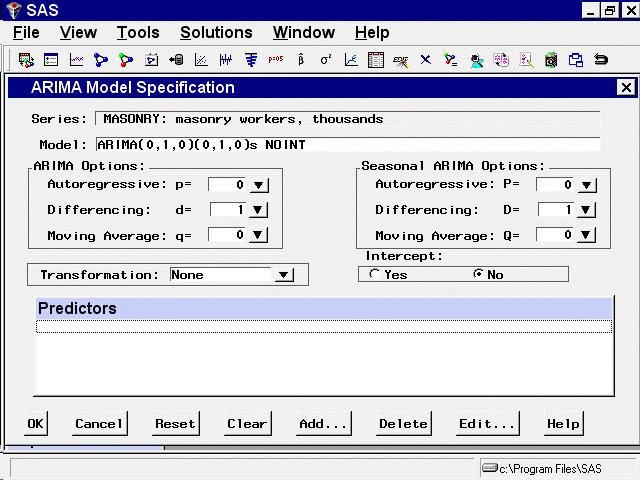
Leave the Time Series Viewer open for the remainder of this exercise. Drag it out of the way or push it to the background so that you can return to the Time Series Forecasting window. Select Develop Models, then click an empty part of the table to bring up the pop-up menu, and select Fit ARIMA Model. Define the ARIMA(0,1,0)(0,1,0)s model by selecting 1 for Differencing under ARIMA Options, 1 for Differencing under Seasonal ARIMA Options, and No for Intercept, as shown in Figure 42.8.

Figure 42.8 Specifying the ARIMA(0,1,0)(0,1,0)s Model

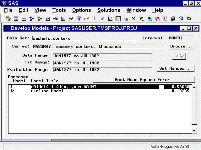
When you select the OK button, the model is fit and you are returned to the Develop Models window. Click on an empty part of the table and choose Fit Models from List from the pop-up menu. Select Airline Model from the window. (Airline Model is a common name for the ARIMA(0,1,1)(0,1,1)s model, which is often used for seasonal data with a linear trend.) Select the OK button. Once the model has been fit, the table shows the two models and their root mean square errors. Notice that the Airline Model provides only a slight improvement over the differencing model, ARIMA(0,1,0)(0,1,0)s. Select the first row to highlight the differencing model, as shown in Figure 42.9.

Figure 42.9 Selecting a Model

Now select the View Selected Model Graphically button, below the Browse button at the right side of the Develop Models window. The Model Viewer window appears, showing the actual data and model predictions for the MASONRY series. (Note that predicted values are missing for the first 13 observations due to simple and seasonal differencing.)

To examine the ACF plot for the model prediction errors, select the third icon from the top on the vertical toolbar. For this model, the prediction error ACF is the same as the ACF of the original data with first differencing and seasonal differencing applied. This differencing is apparent if you bring the Time Series Viewer back into view for comparison.

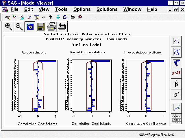
Return to the Develop Models Window by clicking on it or using the window pull-down menu or the Next Viewer toolbar icon. Select the second row of the table in the Develop Models window to highlight the Airline Model. The Model Viewer is automatically updated to show the prediction error ACF of the newly selected model, as shown in Figure 42.10.

Figure 42.10 Prediction Error ACF Plot for the Airline Model

Another helpful tool available within the Model Viewer is the parameter estimates table. Select the fifth icon from the top of the vertical toolbar. The table gives the parameter estimates for the two moving-average terms in the Airline Model, as well as the model residual variance, as shown in Figure 42.11.

Figure 42.11 Parameter Estimates for the Airline Model

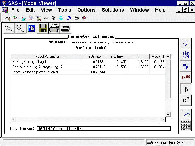
You can adjust the column widths in the table by dragging the vertical borders of the column titles with the mouse. Notice that neither of the parameter estimates is significantly different from zero at the 0.05 level of significance, since Prob>|t| is greater than 0.05. This suggests that the Airline Model should be discarded in favor of the more parsimonious differencing model, which has no parameters to estimate.