| The STATESPACE Procedure |
| Preliminary Autoregressive Models |
After computing the sample autocovariance matrices, PROC STATESPACE fits a sequence of vector autoregressive models. These preliminary autoregressive models are used to estimate the autoregressive order of the process and limit the order of the autocovariances considered in the state vector selection process.
Yule-Walker Equations for Forward and Backward Models
Unlike a univariate autoregressive model, a multivariate autoregressive model has different forms, depending on whether the present observation is being predicted from the past observations or from the future observations.
Let  be the r-component stationary time series given by the VAR statement after differencing and subtracting the vector of sample means. (If the NOCENTER option is specified, the mean is not subtracted.) Let n be the number of observations of from the input data set.
Let  be a vector white noise sequence with mean vector 0 and variance matrix
  , and let
  be a vector white noise sequence with mean vector 0 and variance matrix
  . Let p be the order of the vector autoregressive model for .
The forward autoregressive form based on the past observations is written as follows:
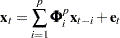 |
The backward autoregressive form based on the future observations is written as follows:
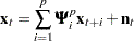 |
Letting  denote the expected value operator, the autocovariance sequence for the series,
  , is
, is
 |
The Yule-Walker equations for the autoregressive model that matches the first p elements of the autocovariance sequence are
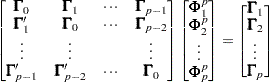 |
and
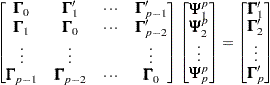 |
Here  are the coefficient matrices for the past observation form of the vector autoregressive model, and
  are the coefficient matrices for the future observation form. More information about the Yule-Walker equations in the multivariate setting can be found in Whittle (1963) and Ansley and Newbold (1979).
The innovation variance matrices for the two forms can be written as follows:
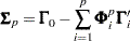 |
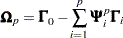 |
The autoregressive models are fit to the data by using the preceding Yule-Walker equations with replaced by the sample covariance sequence  . The covariance matrices are calculated as
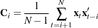 |
Let  ,
,  ,
,  , and
, and  represent the Yule-Walker estimates of
  ,
,  , , and , respectively. These matrices are written to an output data set when the OUTAR= option is specified.
When the PRINTOUT=LONG option is specified, the sequence of matrices and the corresponding correlation matrices are printed. The sequence of matrices is used to compute Akaike information criteria for selection of the autoregressive order of the process.
Akaike Information Criterion
The Akaike information criterion (AIC) is defined as –2(maximum of log likelihood )+2(number of parameters). Since the vector autoregressive models are estimates from the Yule-Walker equations, not by maximum likelihood, the exact likelihood values are not available for computing the AIC. However, for the vector autoregressive model the maximum of the log likelihood can be approximated as
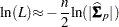 |
Thus, the AIC for the order p model is computed as
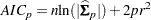 |
You can use the printed AIC array to compute a likelihood ratio test of the autoregressive order. The log-likelihood ratio test statistic for testing the order p model against the order  model is
 |
This quantity is asymptotically distributed as a  with
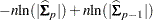
with  degrees of freedom if the series is autoregressive of order . It can be computed from the AIC array as
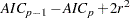 |
You can evaluate the significance of these test statistics with the PROBCHI function in a SAS DATA step or with a table.
Determining the Autoregressive Order
Although the autoregressive models can be used for prediction, their primary value is to aid in the selection of a suitable portion of the sample covariance matrix for use in computing canonical correlations. If the multivariate time series is of autoregressive order p, then the vector of past values to lag p is considered to contain essentially all the information relevant for prediction of future values of the time series.
By default, PROC STATESPACE selects the order p that produces the autoregressive model with the smallest  . If the value p for the minimum is less than the value of the PASTMIN= option, then p is set to the PASTMIN= value. Alternatively, you can use the ARMAX= and PASTMIN= options to force PROC STATESPACE to use an order you select.
Significance Limits for Partial Autocorrelations
The STATESPACE procedure prints a schematic representation of the partial autocorrelation matrices that indicates which partial autocorrelations are significantly greater than or significantly less than 0. Figure 26.11 shows an example of this table.
The partial autocorrelations are from the sample partial autoregressive matrices  . The standard errors used for the significance limits of the partial autocorrelations are computed from the sequence of matrices and .
Under the assumption that the observed series arises from an autoregressive process of order , the pth sample partial autoregressive matrix has an asymptotic variance matrix  .
.
The significance limits for used in the schematic plot of the sample partial autoregressive sequence are derived by replacing and with their sample estimators to produce the variance estimate, as follows:
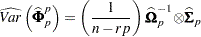 |
Copyright © SAS Institute, Inc. All Rights Reserved.