To perform a Monte Carlo analysis of models that have residuals distributed as a multivariate t, use the ERRORMODEL statement with either the t(variance, df) option or with the CDF=t(variance, df) option. The CDF= option specifies the distribution that is used for simulation so that the estimation can be done for one set of distributional assumptions and the simulation for another.

The following is an example of estimating and simulating a system of equations with t distributed errors by using the ERRORMODEL statement.

/* generate simulation data set */
data five;
   set xfrate end=last;
   if last then do;
      todate = date +5;
      do date = date to todate;
         output;
      end;
   end;
run;

The preceding DATA step generates the data set to request a five-days-ahead forecast. The following statements estimate and forecast the three forward-rate models of the following form.

title "Daily Multivariate Geometric Brownian Motion Model "
         "of D-Mark/USDollar Forward Rates";

proc model data=xfrate;

   parms df 15;       /* Give initial value to df */

   demusd1m = lag(demusd1m) + mu1m * lag(demusd1m);
   var_demusd1m = sigma1m ** 2 * lag(demusd1m **2);
   demusd3m = lag(demusd3m) + mu3m * lag(demusd3m);
   var_demusd3m = sigma3m ** 2 * lag(demusd3m ** 2);
   demusd6m = lag(demusd6m) + mu6m * lag(demusd6m);
   var_demusd6m = sigma6m ** 2 * lag(demusd6m ** 2);

      /* Specify the error distribution */
   errormodel demusd1m demusd3m demusd6m
        ~ t( var_demusd1m var_demusd3m var_demusd6m, df );

      /* output normalized S matrix */
   fit demusd1m demusd3m demusd6m / outsn=s;
run;
      /* forecast five days in advance */
   solve demusd1m demusd3m demusd6m /
         data=five sdata=s random=1500 out=monte;
   id date;
run;

   /* select out the last date ---*/
data monte; set monte;
   if date = '10dec95'd then output;
run;

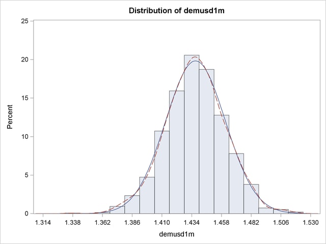
title "Distribution of demusd1m Five Days Ahead";
proc univariate data=monte noprint;
   var demusd1m;
   histogram demusd1m /
             normal(noprint color=red)
             kernel(noprint color=blue) cfill=ligr;
run;

The Monte Carlo simulation specified in the preceding example draws from a multivariate t distribution with constant degrees of freedom and forecasted variance, and it computes future states of DEMUSD1M, DEMUSD3M, and DEMUSD6M. The OUTSN= option in the FIT statement is used to specify the data set for the normalized matrix. That is, the matrix is created by crossing the normally distributed residuals. The normally distributed residuals are created from the t distributed residuals by using the normal inverse CDF and the t CDF. This matrix is a correlation matrix.

The distribution of DEMUSD1M on the fifth day is shown in the Figure 18.70. The two curves overlaid on the graph are a kernel density estimation and a normal distribution fit to the results.

Figure 18.70 Distribution of DEMUSD1M