| The MODEL Procedure |
| Monte Carlo Simulation |
The RANDOM= option is used to request Monte Carlo (or stochastic) simulation to generate confidence intervals for a forecast. The confidence intervals are implied by the model’s relationship to implicit random error term  and the parameters.
The Monte Carlo simulation generates a random set of additive error values, one for each observation and each equation, and computes one set of perturbations of the parameters. These new parameters, along with the additive error terms, are then used to compute a new forecast that satisfies this new simultaneous system. Then a new set of additive error values and parameter perturbations is computed, and the process is repeated the requested number of times.
Consider the following exchange rate model for the U.S. dollar with the German mark and the Japanese yen:
 |
 |
where  and
and  are the exchange rate of the Japanese yen and the German mark versus the U.S. dollar, respectively; im_jp and im_wg are the imports from Japan and Germany in 1984 dollars, respectively; and di_jp and di_wg are the differences in inflation rate of Japan and the U.S., and Germany and the U.S., respectively. The Monte Carlo capabilities of the MODEL procedure are used to generate error bounds on a forecast by using this model.
proc model data=exchange;
   endo im_jp im_wg;
   exo di_jp di_wg;
   parms a1 a2 b1 b2 c1 c2;
   label rate_jp = 'Exchange Rate of Yen/$'
         rate_wg = 'Exchange Rate of Gm/$'
         im_jp = 'Imports to US from Japan in 1984 $'
         im_wg = 'Imports to US from WG in 1984 $'
         di_jp = 'Difference in Inflation Rates US-JP'
         di_wg = 'Difference in Inflation Rates US-WG';

   rate_jp = a1 + b1*im_jp + c1*di_jp;
   rate_wg = a2 + b2*im_wg + c2*di_wg;

            /* Fit the EXCHANGE data */
   fit rate_jp rate_wg / sur outest=xch_est outcov outs=s;

            /* Solve using the WHATIF data set */
   solve rate_jp rate_wg / data=whatif estdata=xch_est sdata=s
          random=100 seed=123 out=monte forecast;
   id yr;
   range yr=1986;
run;
Data for the EXCHANGE data set was obtained from the Department of Commerce and the yearly "Economic Report of the President."
First, the parameters are estimated using SUR selected by the SUR option in the FIT statement. The OUTEST= option is used to create the XCH_EST data set which contains the estimates of the parameters. The OUTCOV option adds the covariance matrix of the parameters to the XCH_EST data set. The OUTS= option is used to save the covariance of the equation error in the data set S.
Next, Monte Carlo simulation is requested by using the RANDOM= option in the SOLVE statement. The data set WHATIF is used to drive the forecasts. The ESTDATA= option reads in the XCH_EST data set which contains the parameter estimates and covariance matrix. Because the parameter covariance matrix is included, perturbations of the parameters are performed. The SDATA= option causes the Monte Carlo simulation to use the equation error covariance in the S data set to perturb the equation errors. The SEED= option selects the number 123 as a seed value for the random number generator. The output of the Monte Carlo simulation is written to the data set MONTE selected by the OUT= option.
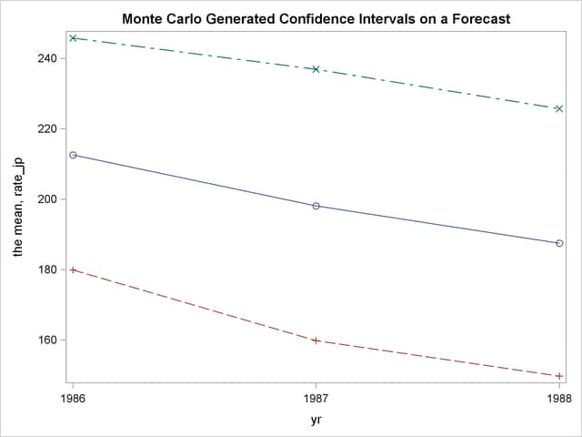
To generate a confidence interval plot for the forecast, use PROC UNIVARIATE to generate percentile bounds and use PROC SGPLOT to plot the graph. The following SAS statements produce the graph in Figure 18.12.
proc sort data=monte;
   by yr;
run;

proc univariate data=monte noprint;
   by yr;
   var rate_jp rate_wg;
   output out=bounds mean=mean p5=p5 p95=p95;
run;

title "Monte Carlo Generated Confidence Intervals on a Forecast";
proc sgplot data=bounds noautolegend;
  series x=yr y=mean / markers;
  series x=yr y=p5 / markers;
  series x=yr y=p95 / markers;
run;
Copyright © SAS Institute, Inc. All Rights Reserved.