Set Fit Options for Equations

The Set fit options page enables you to estimate model parameters by fitting the model equations to input data and optionally select the equations to be fit.

Figure 47.12 Set Fit Options for an Equation

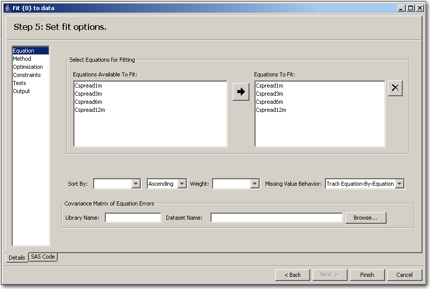
This page has the following controls and fields:

Equations Available to Fit: box

lists the variables in the input data set that you can select to fit equations to.

Equations To Fit: box

lists the variables in the input data set that are selected to fit equations to.

Sort By:

indicates how the fit options are sorted. This field has two list boxes. In the left list box, select the variable by which to sort. In the right list box, select Ascending, Descending, or Not Sorted.

Weight:

specifies a weighting value to apply to each observation when estimating parameters.

Missing Value Behavior:

specifies whether missing values are tracked on an equation-by-equation basis or the entire observation is omitted from the analysis when any equation has a missing predicted or actual value for the equation.

Library Name:

specifies the SAS library where you can select your data set.

Dataset Name:

specifies the selected input data set from the SAS library you would like to work on.

Browse button

opens the data set selection window for selecting an input data set.

Set Fit Options for a Method

This page enables you to choose how the parameters are to be estimated. See Chapter 18, "The MODEL Procedure" (SAS/ETS User’s Guide), for more information about available methods of parameter estimation.

Figure 47.13 Set Fit Options for a Method

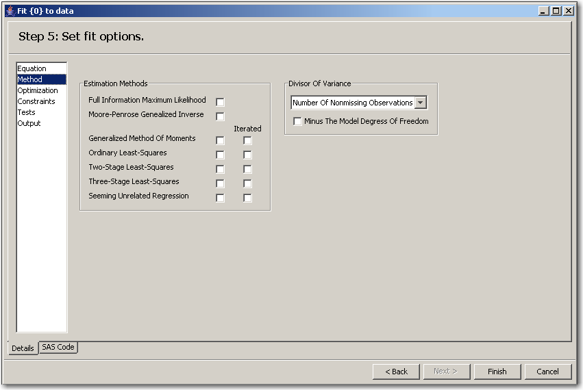
This page has the following controls and fields:

Estimation Methods check boxes

enable you to select the corresponding estimation method. All of the methods implemented in PROC MODEL aim to minimize an objective function.

The following methods for parameter estimation can be selected (the equivalent MODEL procedure option is shown in parentheses):

• Full Information Maximum Likelihood (FIML)

• Moore-Penrose Generalized Inverse (MPGI)

• Generalized Method of Moments (GMM)

• Iterated Generalized Method of Moments (ITGMM)

• Ordinary Least Squares (OLS) (This is the default.)

• Iterated Ordinary Least Squares (ITOLS)

• Two-Stage Least Squares (2SLS)

• Iterated Two-Stage Least Squares (IT2SLS)

• Three-Stage Least Squares (3SLS)

• Iterated Three-Stage Least Squares (IT3SLS)

• Seemingly Unrelated Regression (SUR)

• Iterated Seemingly Unrelated Regression (ITSUR)

When Estimation Method for GMM or ITGMM check boxes are selected, additional fields are displayed. These fields correspond to options used in the kernel options in MODEL procedure. You can specify kernel options such as Parzen, Bartlett, and quadratic spectral. For more information about KERNEL options, see Chapter 18, "The MODEL Procedure" (SAS/ETS User’s Guide).

Divisor of Variance

specifies a degrees-of-freedom correction in estimating the variance matrix. This could be the sum of the weights or the sum of the weights minus the model degrees of freedom.

Set Fit Options for an Optimization

This page provides an interface for controlling the objective function minimization process and the integration process. If you encounter difficulty in achieving convergence, then changing the settings of one or more of the process control options might assist in achieving convergence. Except for the Method, the templates are numeric. Type the appropriate value into the text boxes.

Note:If you have not been given permission to edit the model, you can only browse the minimization and integration process options.

Figure 47.14 Set Fit Options for an Optimation

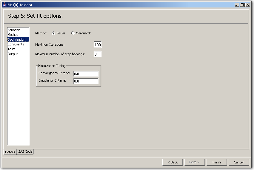
This page has the following controls and fields:

Method: options

specifies the Gauss method or Marquardt method. Gauss is the default.

For the Gauss method, the Gauss-Newton parameter-change vector for a system is computed at the end of each iteration. The objective function is then computed at the changed parameter values at the start of the next iteration. For the Marquardt method, at each iteration, the objective function is evaluated at the parameters changed by the Marquardt-Levenberg parameter-change vector. For information about available methods of parameter estimation, see Chapter 18, "The MODEL Procedure," (SAS/ETS User’s Guide).

Maximum Iterations:

specifies the maximum number of Newton iterations performed at each observation and each replication of Monte Carlo simulations.

Maximum number of step halvings:

specifies the maximum number of subiterations allowed for an iteration. For the Gauss method, this value limits the number of step halvings. For the Marquardt method, this value limits the number of times the step parameter can be increased. The default is MAXSUBITER=30. See Chapter 18, "The MODEL Procedure" (SAS/ETS User’s Guide), for more information.

Minimization Tuning

specifies the Convergence Criteria and Singularity Criteria.

Set Fit Options for Constraints

This page lists any previously defined constraints for the model. Initially, there are no constraints defined.

Figure 47.15 Set Fit Options for Constraints

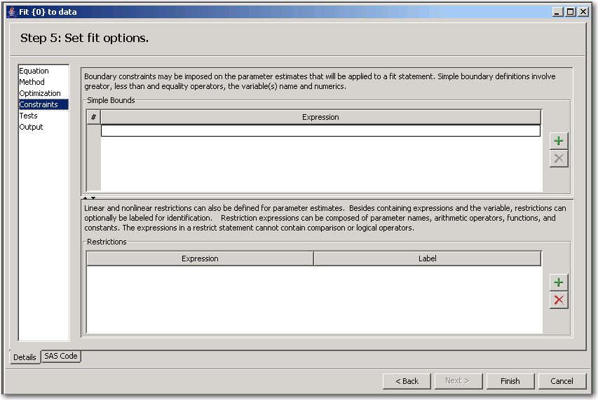
This page has the following controls and fields:

Simple Bounds

impose simple boundary constraints on the parameter estimates. You can specify any number of statements in this field. To add a new constraint, click the Add button .

Restrictions

impose linear and nonlinear restrictions on the parameter estimates. You can use both Simple Bounds statements and Restrictions statements to impose boundary constraints. However, the Simple Bounds statements provide a simpler syntax for specifying these kinds of constraints.

Suppose you want to restrict the parameter that is associated with the first exogenous (independent) variable to be greater than zero (0). To add this parameter restriction to the model template, click the Add button . If the restriction code contains syntax errors, an error dialog box appears that has instructions for correcting the restriction code.

Set Fit Options for Tests

This page enables you to perform tests of nonlinear hypotheses on the model parameters. You can define statistical tests that are associated with the model parameters. This page lists any previously defined parameter tests for the model. Initially, there are no tests defined.

Figure 47.16 Set Fit Options for Tests

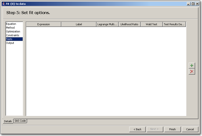
This page has the following controls and fields:

Tests

perform tests of nonlinear hypotheses on the model parameters. Test expressions can be composed of parameter names, arithmetic operators, functions, and constants. You can specify any number of test statements by typing the test equations in this page.

Suppose that you want to test that the parameters that are associated with the first and second exogenous (independent) variables are equal. Click the Add button to display the Test Expression equation.

In the Label field, type "My test". In the Expression field, type the following expression: a = b.

The type of test can be Wald, Lagrange multiplier (LM), likelihood ratio (LR), or all three (ALL). To add this test, click the Add button . If the test expression contains syntax errors, an error dialog box appears that has instructions about correcting the test expression. See Chapter 18, "The MODEL Procedure" (SAS/ETS User’s Guide), for more information.

You can define any number of tests.

Set Fit Options for Outputs

Figure 47.17 Set Fit Options for Outputs

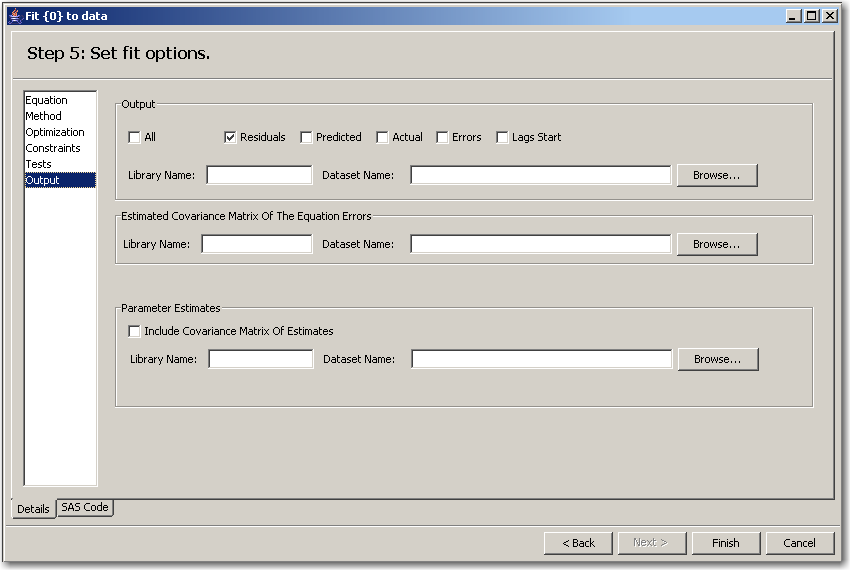
This page has the following controls and fields:

Output

specifies which results to display for your fitted model. Select one or more check boxes (or select All) to indicate which analyses you want to include in the output data set. Select All to display all analyses for each model equation. Select Predicted to show the predicted value of this model. Select Actual to display the actual value of the model. Select Errors to display residual error analysis for each model equation. Select Lags Start to display the lag-starting observations.

Estimated Covariance of the Equation Errors

displays the cross-equation covariance. In addition, the determinant of the matrices is displayed.

Parameter Estimates

displays the parameter estimates. You can show the parameter estimated covariance and correlations matrices by selecting Include Covariance Matrix of Estimates.

Library Name:

is the name of the library where the user-specified output is saved.

Dataset Name:

is the data set in which you want the user-specified output to be saved.

Browse:

opens the data set selection window for selecting an output data set.