| The MDC Procedure |
Example 17.5 Choice of Time for Work Trips: Nested Logit Analysis
This example uses sample data of 527 automobile commuters in the San Francisco Bay Area to demonstrate the use of nested logit model.
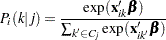
Brownstone and Small (1989) analyzed a two-level nested logit model that is displayed in Figure 17.30. The probability of choosing  at level 2 is written as
 |
where  is an inclusive value and is computed as
 |
The probability of choosing an alternative  is denoted as
 |
The full information maximum likelihood (FIML) method maximizes the following log-likelihood function:
 |
where  if a decision maker
  chooses , and 0 otherwise.
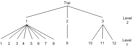
Sample data of 527 automobile commuters in the San Francisco Bay Area have been analyzed by Small (1982) and Brownstone and Small (1989). The regular time of arrival is recorded as between 42.5 minutes early and 17.5 minutes late, and indexed by 12 alternatives, using five-minute interval groups. Refer to Small (1982) for more details on these data.
The following statements estimate the two-level nested logit model:
/*-- Two-level Nested Logit --*/
proc mdc data=small maxit=200 outest=a;
   model decision = r15 r10 ttime ttime_cp sde sde_cp
                    sdl sdlx d2l /
            type=nlogit
            choice=(alt);
   id id;
   utility u(1, ) = r15 r10 ttime ttime_cp sde sde_cp
                    sdl sdlx d2l;
   nest level(1) = (1 2 3 4 5 6 7 8 @ 1, 9 @ 2, 10 11 12 @ 3),
        level(2) = (1 2 3 @ 1);
run;
The estimation summary, discrete response profile, and the FIML estimates are displayed in Output 17.5.1 through Output 17.5.3.
| Model Fit Summary | |
|---|---|
| Dependent Variable | decision |
| Number of Observations | 527 |
| Number of Cases | 6324 |
| Log Likelihood | -990.81912 |
| Log Likelihood Null (LogL(0)) | -1310 |
| Maximum Absolute Gradient | 4.93868E-6 |
| Number of Iterations | 18 |
| Optimization Method | Newton-Raphson |
| AIC | 2006 |
| Schwarz Criterion | 2057 |
| Parameter Estimates | |||||
|---|---|---|---|---|---|
| Parameter | DF | Estimate | Standard Error |
t Value | Approx Pr > |t| |
| r15_L1 | 1 | 1.1034 | 0.1221 | 9.04 | <.0001 |
| r10_L1 | 1 | 0.3931 | 0.1194 | 3.29 | 0.0010 |
| ttime_L1 | 1 | -0.0465 | 0.0235 | -1.98 | 0.0474 |
| ttime_cp_L1 | 1 | -0.0498 | 0.0305 | -1.63 | 0.1028 |
| sde_L1 | 1 | -0.6618 | 0.0833 | -7.95 | <.0001 |
| sde_cp_L1 | 1 | 0.0519 | 0.1278 | 0.41 | 0.6850 |
| sdl_L1 | 1 | -2.1006 | 0.5062 | -4.15 | <.0001 |
| sdlx_L1 | 1 | -3.5240 | 1.5346 | -2.30 | 0.0217 |
| d2l_L1 | 1 | -1.0941 | 0.3273 | -3.34 | 0.0008 |
| INC_L2G1C1 | 1 | 0.6762 | 0.2754 | 2.46 | 0.0141 |
| INC_L2G1C2 | 1 | 1.0906 | 0.3090 | 3.53 | 0.0004 |
| INC_L2G1C3 | 1 | 0.7622 | 0.1649 | 4.62 | <.0001 |
Now policy makers are particularly interested in predicting shares of each alternative to be chosen by population. One application of such predictions are market shares. Going even further, it is extremely useful to predict choice probabilities out of sample; that is, under alternative policies.
Suppose that in this particular transportation example you are interested in projecting the effect of a new program that indirectly shifts individual preferences with respect to late arrival to work. This means that you manage to decrease the coefficient for the “late dummy” D2L, which is a penalty for violating some margin of arriving on time. Suppose that you alter it from an estimated  to almost twice that level,
  .
.
But first, in order to have a benchmark share, you predict probabilities to choose each particular option and output them to the new data set with the following additional statement:
/*-- Create new data set with predicted probabilities --*/
output out=predicted1 p=probs;
Having these in sample predictions, you sort the data by alternative and aggregate across each of them as shown in the following statements:
/*-- Sort the data by alternative --*/
proc sort data=predicted1;
   by alt;
run;

/*-- Calculate average probabilities of each alternative --*/
proc means data=predicted1 noobs mean;
   var probs;
   class alt;
run;
Output 17.5.4 shows the summary table that is produced by the preceding statements.
| Analysis Variable : probs | |
|---|---|
| alt | Mean |
| 1 | 0.0178197 |
| 2 | 0.0161712 |
| 3 | 0.0972584 |
| 4 | 0.0294659 |
| 5 | 0.0594076 |
| 6 | 0.1653871 |
| 7 | 0.1118181 |
| 8 | 0.1043445 |
| 9 | 0.3564940 |
| 10 | 0.0272324 |
| 11 | 0.0096334 |
| 12 | 0.0049677 |
Now you change the preference parameter for variable D2L. In order to fix all the parameters, you use the MAXIT=0 option to prevent optimization and the START= option in MODEL statement to specify initial parameters.
/*-- Two-level Nested Logit --*/
proc mdc data=small maxit=0 outest=a;
   model decision = r15 r10 ttime ttime_cp sde sde_cp
                    sdl sdlx d2l /
            type=nlogit
            choice=(alt)
            start=( 1.1034 0.3931 -0.0465 -0.0498
                   -0.6618 0.0519 -2.1006 -3.5240
                   -2.0941 0.6762  1.0906  0.7622);
   id id;
   utility u(1, ) = r15 r10 ttime ttime_cp sde sde_cp
                    sdl sdlx d2l;
   nest level(1) = (1 2 3 4 5 6 7 8 @ 1, 9 @ 2, 10 11 12 @ 3),
        level(2) = (1 2 3 @ 1);
   output out=predicted2 p=probs;
run;
You apply the same SORT and MEANS procedures as applied earlier to obtain the following summary table in Output 17.5.5.
| Analysis Variable : probs | |
|---|---|
| alt | Mean |
| 1 | 0.0207766 |
| 2 | 0.0188966 |
| 3 | 0.1138816 |
| 4 | 0.0345654 |
| 5 | 0.0697830 |
| 6 | 0.1944572 |
| 7 | 0.1315588 |
| 8 | 0.1228049 |
| 9 | 0.2560674 |
| 10 | 0.0236178 |
| 11 | 0.0090781 |
| 12 | 0.0045128 |
Comparing the two tables shown in Output 17.5.4 and Output 17.5.5, you clearly see the effect of increased dislike of late arrival. People shifted their choices towards earlier times (alternatives 1–8) from the on-time option (alternative 9).
Brownstone and Small (1989) also estimate the two-level nested logit model with equal scale parameter constraints,  . Replication of their model estimation is shown in the following statements:
/*-- Nested Logit with Equal Dissimilarity Parameters --*/
proc mdc data=small maxit=200 outest=a;
   model decision = r15 r10 ttime ttime_cp sde sde_cp
                    sdl sdlx d2l /
            samescale
            type=nlogit
            choice=(alt);
   id id;
   utility u(1, ) = r15 r10 ttime ttime_cp sde sde_cp
                    sdl sdlx d2l;
   nest level(1) = (1 2 3 4 5 6 7 8 @ 1, 9 @ 2, 10 11 12 @ 3),
        level(2) = (1 2 3 @ 1);
run;
The parameter estimates and standard errors are almost identical to those in Brownstone and Small (1989, p. 69). Output 17.5.6 and Output 17.5.7 display the results.
| Model Fit Summary | |
|---|---|
| Dependent Variable | decision |
| Number of Observations | 527 |
| Number of Cases | 6324 |
| Log Likelihood | -994.39402 |
| Log Likelihood Null (LogL(0)) | -1310 |
| Maximum Absolute Gradient | 2.97172E-6 |
| Number of Iterations | 16 |
| Optimization Method | Newton-Raphson |
| AIC | 2009 |
| Schwarz Criterion | 2051 |
| Parameter Estimates | |||||
|---|---|---|---|---|---|
| Parameter | DF | Estimate | Standard Error |
t Value | Approx Pr > |t| |
| r15_L1 | 1 | 1.1345 | 0.1092 | 10.39 | <.0001 |
| r10_L1 | 1 | 0.4194 | 0.1081 | 3.88 | 0.0001 |
| ttime_L1 | 1 | -0.1626 | 0.0609 | -2.67 | 0.0076 |
| ttime_cp_L1 | 1 | 0.1285 | 0.0853 | 1.51 | 0.1319 |
| sde_L1 | 1 | -0.7548 | 0.0669 | -11.28 | <.0001 |
| sde_cp_L1 | 1 | 0.2292 | 0.0981 | 2.34 | 0.0195 |
| sdl_L1 | 1 | -2.0719 | 0.4860 | -4.26 | <.0001 |
| sdlx_L1 | 1 | -2.8216 | 1.2560 | -2.25 | 0.0247 |
| d2l_L1 | 1 | -1.3164 | 0.3474 | -3.79 | 0.0002 |
| INC_L2G1 | 1 | 0.8059 | 0.1705 | 4.73 | <.0001 |
However, the test statistic for  rejects the null hypothesis at the
  significance level since
  . The
. The  -value is computed in the following statements and is equal to
  :
:
data _null_;
   /*-- test for H0: tau1 = tau2 = tau3 --*/
   /*   ln L(max) = -990.8191             */
   /*   ln L(0)   = -994.3940             */
   stat = -2 * ( -994.3940 + 990.8191 );
   df = 2;
   p_value = 1 - probchi(stat, df);
   put stat= p_value=;
run;
Copyright © SAS Institute, Inc. All Rights Reserved.