Suppose a rock quarry needs equipment to use the next five years. It has two alternatives:

• a box loader and conveyer system that has a one-time cost of $264,000

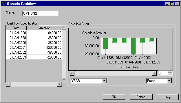
• a two-shovel loader, which costs $84,000 but has a yearly operating cost of $36,000. This loader has a service life of three years, which necessitates the purchase of a new loader for the final two years of the rock quarry project. Assume the second loader also costs $84,000 and its salvage value after its two-year service is $10,000. A SAS data set that describes this is available at SASHELP.ROCKPIT

You expect a 13% MARR. Which is the better alternative?

To create the cashflows, follow these steps:

1. Create a cashflow with the single amount –264,000. Date the amount 01JAN1998 to be consistent with the SAS data set you load.

2. Load SASHELP.ROCKPIT into a second cashflow, as displayed in Figure 52.2.

Figure 52.2 The contents of SASHELP.ROCKPIT

To compute the time values of these investments, follow these steps:

1. Select both cashflows.

2. Select Analyze Time Value. This opens the Time Value Analysis dialog box.

3. Enter the date 01JAN1998 into the Dates area.

4. Enter 13 for the Constant MARR.

5. Click Create Time Value Summary.

Figure 52.3 Performing the Time Value Analysis

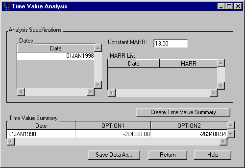
As shown in Figure 52.3, option 1 has a time value of –$264,000.00 naturally on 01JAN1998. However, option 2 has a time value of –$263,408.94, which is slightly less expensive.