| The ARIMA Procedure |
Example 7.3 Model for Series J Data from Box and Jenkins
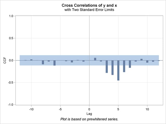
This example uses the Series J data from Box and Jenkins (1976). First, the input series X is modeled with a univariate ARMA model. Next, the dependent series Y is cross-correlated with the input series. Since a model has been fit to X, both Y and X are prewhitened by this model before the sample cross-correlations are computed. Next, a transfer function model is fit with no structure on the noise term. The residuals from this model are analyzed; then, the full model, transfer function and noise, is fit to the data.
The following statements read 'Input Gas Rate' and 'Output CO ' from a gas furnace. (Data values are not shown. The full example including data is in the SAS/ETS sample library.)
title1 'Gas Furnace Data';
title2 '(Box and Jenkins, Series J)';
data seriesj;
   input x y @@;
   label x = 'Input Gas Rate'
         y = 'Output CO2';
datalines;

   ... more lines ...
The following statements produce Output 7.3.1 through Output 7.3.11:
ods graphics on;
proc arima data=seriesj;

   /*--- Look at the input process -------------------*/
   identify var=x;
   run;

   /*--- Fit a model for the input -------------------*/
   estimate p=3 plot;
   run;

   /*--- Crosscorrelation of prewhitened series ------*/
   identify var=y crosscorr=(x) nlag=12;
   run;

   /*- Fit a simple transfer function - look at residuals -*/
   estimate input=( 3 $ (1,2)/(1) x );
   run;

   /*--- Final Model - look at residuals ---*/
   estimate p=2 input=( 3 $ (1,2)/(1) x );
   run;

quit;
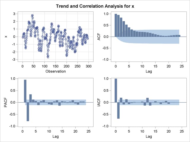
The results of the first IDENTIFY statement for the input series X are shown in Output 7.3.1. The correlation analysis suggests an AR(3) model.
| Name of Variable = x | |
|---|---|
| Mean of Working Series | -0.05683 |
| Standard Deviation | 1.070952 |
| Number of Observations | 296 |
The ESTIMATE statement results for the AR(3) model for the input series X are shown in Output 7.3.3.
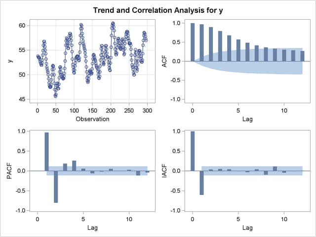
The IDENTIFY statement results for the dependent series Y cross-correlated with the input series X are shown in Output 7.3.4, Output 7.3.5, Output 7.3.6, and Output 7.3.7. Since a model has been fit to X, both Y and X are prewhitened by this model before the sample cross-correlations are computed.
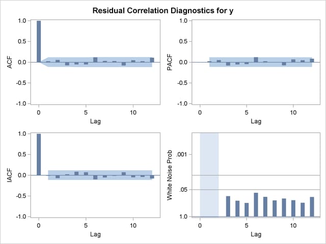
The ESTIMATE statement results for the transfer function model with no structure on the noise term are shown in Output 7.3.8, Output 7.3.9, and Output 7.3.10.
| Conditional Least Squares Estimation | |||||||
|---|---|---|---|---|---|---|---|
| Parameter | Estimate | Standard Error | t Value | Approx Pr > |t| |
Lag | Variable | Shift |
| MU | 53.32256 | 0.04926 | 1082.51 | <.0001 | 0 | y | 0 |
| NUM1 | -0.56467 | 0.22405 | -2.52 | 0.0123 | 0 | x | 3 |
| NUM1,1 | 0.42623 | 0.46472 | 0.92 | 0.3598 | 1 | x | 3 |
| NUM1,2 | 0.29914 | 0.35506 | 0.84 | 0.4002 | 2 | x | 3 |
| DEN1,1 | 0.60073 | 0.04101 | 14.65 | <.0001 | 1 | x | 3 |
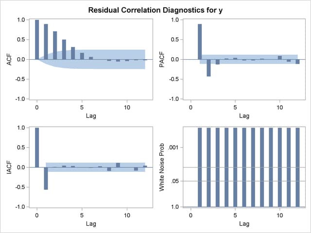
The residual correlation analysis suggests an AR(2) model for the noise part of the model. The ESTIMATE statement results for the final transfer function model with AR(2) noise are shown in Output 7.3.11.
| Conditional Least Squares Estimation | |||||||
|---|---|---|---|---|---|---|---|
| Parameter | Estimate | Standard Error | t Value | Approx Pr > |t| |
Lag | Variable | Shift |
| MU | 53.26304 | 0.11929 | 446.48 | <.0001 | 0 | y | 0 |
| AR1,1 | 1.53291 | 0.04754 | 32.25 | <.0001 | 1 | y | 0 |
| AR1,2 | -0.63297 | 0.05006 | -12.64 | <.0001 | 2 | y | 0 |
| NUM1 | -0.53522 | 0.07482 | -7.15 | <.0001 | 0 | x | 3 |
| NUM1,1 | 0.37603 | 0.10287 | 3.66 | 0.0003 | 1 | x | 3 |
| NUM1,2 | 0.51895 | 0.10783 | 4.81 | <.0001 | 2 | x | 3 |
| DEN1,1 | 0.54841 | 0.03822 | 14.35 | <.0001 | 1 | x | 3 |
Copyright © SAS Institute, Inc. All Rights Reserved.