Example 7.1 Simulated IMA Model

This example illustrates the ARIMA procedure results for a case where the true model is known. An integrated moving-average model is used for this illustration.

The following DATA step generates a pseudo-random sample of 100 periods from the ARIMA(0,1,1) process , :

title1 'Simulated IMA(1,1) Series';
data a;
  u1 = 0.9; a1 = 0;
  do i = -50 to 100;
     a = rannor( 32565 );
     u = u1 + a - .8 * a1;
     if i > 0 then output;
     a1 = a;
     u1 = u;
  end;
run;

The following ARIMA procedure statements identify and estimate the model:

ods graphics on;
/*-- Simulated IMA Model --*/
proc arima data=a;
  identify var=u;
  run;
  identify var=u(1);
  run;
  estimate q=1 ;
  run;
quit;

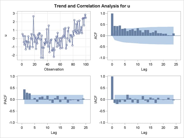
The graphical series correlation analysis output of the first IDENTIFY statement is shown in Output 7.1.1. The output shows the behavior of the sample autocorrelation function when the process is nonstationary. Note that in this case the estimated autocorrelations are not very high, even at small lags. Nonstationarity is reflected in a pattern of significant autocorrelations that do not decline quickly with increasing lag, not in the size of the autocorrelations.

Output 7.1.1 Correlation Analysis from the First IDENTIFY Statement

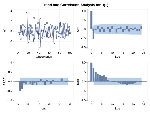
The second IDENTIFY statement differences the series. The results of the second IDENTIFY statement are shown in Output 7.1.2. This output shows autocorrelation, inverse autocorrelation, and partial autocorrelation functions typical of MA(1) processes.

Output 7.1.2 Correlation Analysis from the Second IDENTIFY Statement

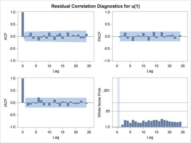
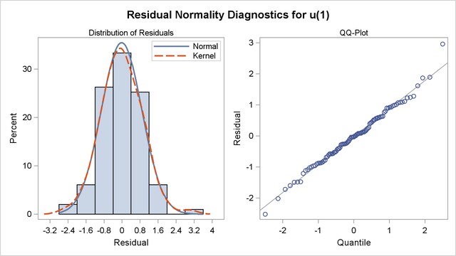
The ESTIMATE statement fits an ARIMA(0,1,1) model to the simulated data. Note that in this case the parameter estimates are reasonably close to the values used to generate the simulated data. () Moreover, the graphical analysis of the residuals shows no model inadequacies (see Output 7.1.4 and Output 7.1.5).

The ESTIMATE statement results are shown in Output 7.1.3.

Output 7.1.4 Residual Correlation Analysis of the ARIMA(0,1,1) Model

Output 7.1.5 Residual Normality Analysis of the ARIMA(0,1,1) Model