| The VARMAX Procedure |
| Multivariate GARCH Modeling |
Stochastic volatility modeling is important in many areas, particularly in finance. To study the volatility of time series, GARCH models are widely used because they provide a good approach to conditional variance modeling.
BEKK Representation
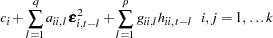
Engle and Kroner (1995) propose a general multivariate GARCH model and call it a BEKK representation. Let  be the sigma field generated by the past values of
  , and let
  be the conditional covariance matrix of the
  -dimensional random vector . Let be measurable with respect to ; then the multivariate GARCH model can be written as
 |
 |
 |
|||
 |
 |
 |
where  ,
,  and
and  are
are  parameter matrices.
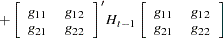
Consider a bivariate GARCH(1,1) model as follows:
 |
 |
 |
|||
 |
|
 |
or, representing the univariate model,
 |
|
 |
|||
|
|
 |
|||
 |
|
 |
|||
|
|
 |
|||
 |
|
 |
|||
|
|
 |
For the BEKK representation of the bivariate GARCH(1,1) model, the SAS statements are:
   model y1 y2;
   garch q=1 p=1 form=bekk;
CCC Representation
Bollerslev (1990) propose a multivariate GARCH model with time-varying conditional variances and covariances but constant conditional correlations.
The conditional covariance matrix consists of
 |
where  is a
is a  stochastic diagonal matrix with element
  and
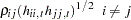
and  is a time-invariant matrix with the typical element
  .
.
The elements of are
 |
|
 |
|||
 |
|
 |
Estimation of GARCH Model
The log-likelihood function of the multivariate GARCH model is written without a constant term
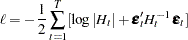 |
The log-likelihood function is maximized by an iterative numerical method such as quasi-Newton optimization. The starting values for the regression parameters are obtained from the least squares estimates. The covariance of  is used as the starting values for the GARCH constant parameters, and the starting value used for the other GARCH parameters is either
  or
or  depending on the GARCH models representation. For the identification of the parameters of a BEKK representation GARCH model, the diagonal elements of the GARCH constant, the ARCH, and the GARCH parameters are restricted to be positive.
Covariance Stationarity
Define the multivariate GARCH process as
 |
where  ,
,  , and
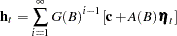
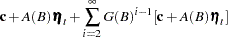
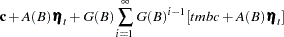
, and  . This representation is equivalent to a GARCH(
 ) model by the following algebra:
 |
|
 |
|||
|
|
 |
|||
|
|
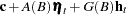 |
Defining 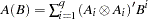 and
and 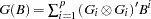 gives a BEKK representation.
The necessary and sufficient conditions for covariance stationarity of the multivariate GARCH process is that all the eigenvalues of  are less than one in modulus.
An Example of a VAR(1)–ARCH(1) Model
The following DATA step simulates a bivariate vector time series to provide test data for the multivariate GARCH model:
   data garch;
      retain seed 16587;
      esq1 = 0; esq2 = 0;
      ly1 = 0;  ly2 = 0;
      do i = 1 to 1000;
         ht = 6.25 + 0.5*esq1;
         call rannor(seed,ehat);
         e1 = sqrt(ht)*ehat;
         ht = 1.25 + 0.7*esq2;
         call rannor(seed,ehat);
         e2 = sqrt(ht)*ehat;
         y1 = 2 + 1.2*ly1 - 0.5*ly2 + e1;
         y2 = 4 + 0.6*ly1 + 0.3*ly2 + e2;
         if i>500 then output;
         esq1 = e1*e1; esq2 = e2*e2;
         ly1 = y1;  ly2 = y2;
      end;
      keep y1 y2;
   run;
The following statements fit a VAR(1)–ARCH(1) model to the data. For a VAR-ARCH model, you specify the order of the autoregressive model with the P=1 option in the MODEL statement and the Q=1 option in the GARCH statement. In order to produce the initial and final values of parameters, the TECH=QN option is specified in the NLOPTIONS statement.
   proc varmax data=garch;
      model y1 y2 / p=1
            print=(roots estimates diagnose);
      garch q=1;
      nloptions tech=qn;
   run;
Figure 30.61 through Figure 30.65 show the details of this example. Figure 30.61 shows the initial values of parameters.
| Optimization Start | |||
|---|---|---|---|
| Parameter Estimates | |||
| N | Parameter | Estimate | Gradient Objective Function |
| 1 | CONST1 | 2.249575 | 5.787988 |
| 2 | CONST2 | 3.902673 | -4.856056 |
| 3 | AR1_1_1 | 1.231775 | -17.155796 |
| 4 | AR1_2_1 | 0.576890 | 23.991176 |
| 5 | AR1_1_2 | -0.528405 | 14.656979 |
| 6 | AR1_2_2 | 0.343714 | -12.763695 |
| 7 | GCHC1_1 | 9.929763 | -0.111361 |
| 8 | GCHC1_2 | 0.193163 | -0.684986 |
| 9 | GCHC2_2 | 4.063245 | 0.139403 |
| 10 | ACH1_1_1 | 0.001000 | -0.668058 |
| 11 | ACH1_2_1 | 0 | -0.068657 |
| 12 | ACH1_1_2 | 0 | -0.735896 |
| 13 | ACH1_2_2 | 0.001000 | -3.126628 |
Figure 30.62 shows the final parameter estimates.
| Optimization Results | ||
|---|---|---|
| Parameter Estimates | ||
| N | Parameter | Estimate |
| 1 | CONST1 | 1.943991 |
| 2 | CONST2 | 4.073898 |
| 3 | AR1_1_1 | 1.220945 |
| 4 | AR1_2_1 | 0.608263 |
| 5 | AR1_1_2 | -0.527121 |
| 6 | AR1_2_2 | 0.303012 |
| 7 | GCHC1_1 | 8.359045 |
| 8 | GCHC1_2 | -0.182483 |
| 9 | GCHC2_2 | 1.602739 |
| 10 | ACH1_1_1 | 0.377569 |
| 11 | ACH1_2_1 | 0.032158 |
| 12 | ACH1_1_2 | 0.056491 |
| 13 | ACH1_2_2 | 0.710023 |
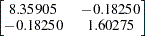
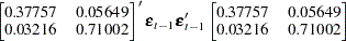
Figure 30.63 shows the conditional variance using the BEKK representation of the ARCH(1) model. The ARCH parameters are estimated by the vectorized parameter matrices.
|
|
|
|||
|
|
 |
|||
|
 |
 |
| Type of Model | VAR(1)-ARCH(1) |
|---|---|
| Estimation Method | Maximum Likelihood Estimation |
| Representation Type | BEKK |
| GARCH Model Parameter Estimates | ||||
|---|---|---|---|---|
| Parameter | Estimate | Standard Error |
t Value | Pr > |t| |
| GCHC1_1 | 8.35905 | 0.73116 | 11.43 | 0.0001 |
| GCHC1_2 | -0.18248 | 0.21706 | -0.84 | 0.4009 |
| GCHC2_2 | 1.60274 | 0.19398 | 8.26 | 0.0001 |
| ACH1_1_1 | 0.37757 | 0.07470 | 5.05 | 0.0001 |
| ACH1_2_1 | 0.03216 | 0.06971 | 0.46 | 0.6448 |
| ACH1_1_2 | 0.05649 | 0.02622 | 2.15 | 0.0317 |
| ACH1_2_2 | 0.71002 | 0.06844 | 10.37 | 0.0001 |
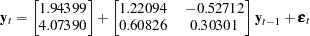
Figure 30.64 shows the AR parameter estimates and their significance.
The fitted VAR(1) model with the previous conditional covariance ARCH model is written as follows:
 |
| Model Parameter Estimates | ||||||
|---|---|---|---|---|---|---|
| Equation | Parameter | Estimate | Standard Error |
t Value | Pr > |t| | Variable |
| y1 | CONST1 | 1.94399 | 0.21017 | 9.25 | 0.0001 | 1 |
| AR1_1_1 | 1.22095 | 0.02564 | 47.63 | 0.0001 | y1(t-1) | |
| AR1_1_2 | -0.52712 | 0.02836 | -18.59 | 0.0001 | y2(t-1) | |
| y2 | CONST2 | 4.07390 | 0.10574 | 38.53 | 0.0001 | 1 |
| AR1_2_1 | 0.60826 | 0.01231 | 49.42 | 0.0001 | y1(t-1) | |
| AR1_2_2 | 0.30301 | 0.01498 | 20.23 | 0.0001 | y2(t-1) | |
Figure 30.65 shows the roots of the AR and ARCH characteristic polynomials. The eigenvalues have a modulus less than one.
| Roots of AR Characteristic Polynomial | |||||
|---|---|---|---|---|---|
| Index | Real | Imaginary | Modulus | Radian | Degree |
| 1 | 0.76198 | 0.33163 | 0.8310 | 0.4105 | 23.5197 |
| 2 | 0.76198 | -0.33163 | 0.8310 | -0.4105 | -23.5197 |
| Roots of GARCH Characteristic Polynomial | |||||
|---|---|---|---|---|---|
| Index | Real | Imaginary | Modulus | Radian | Degree |
| 1 | 0.51180 | 0.00000 | 0.5118 | 0.0000 | 0.0000 |
| 2 | 0.26627 | 0.00000 | 0.2663 | 0.0000 | 0.0000 |
| 3 | 0.26627 | 0.00000 | 0.2663 | 0.0000 | 0.0000 |
| 4 | 0.13853 | 0.00000 | 0.1385 | 0.0000 | 0.0000 |
Copyright © 2008 by SAS Institute Inc., Cary, NC, USA. All rights reserved.