| The VARMAX Procedure |
| VARMA and VARMAX Modeling |
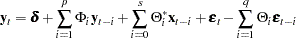
A VARMA( ) process is written as
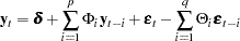 |
or
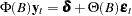 |
where 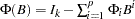 and
and 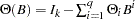 .
.
Stationarity and Invertibility
For stationarity and invertibility of the VARMA process, the roots of  and
and  are outside the unit circle.
Parameter Estimation
Under the assumption of normality of the  with mean vector zero and nonsingular covariance matrix
  , consider the conditional (approximate) log-likelihood function of a VARMA(
 ,
, ) model with mean zero.
Define  and
and  with
with  and
and  ; define
  and
and  . Then
 |
where 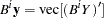 and
and 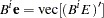 .
.
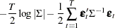
Then, the conditional (approximate) log-likelihood function can be written as follows (Reinsel 1997):
 |
 |
 |
|||
 |
|
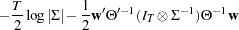 |
where 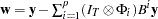 , and
, and  is such that
 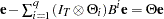 .
.
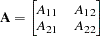
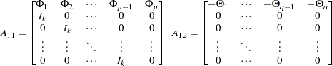
For the exact log-likelihood function of a VARMA(,) model, the Kalman filtering method is used transforming the VARMA process into the state-space form (Reinsel 1997).
The state-space form of the VARMA(,) model consists of a state equation
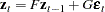 |
and an observation equation
 |
where for 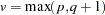
 |
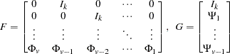 |
and
 |
The Kalman filtering approach is used for evaluation of the likelihood function. The updating equation is
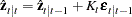 |
with
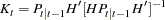 |
and the prediction equation is
 |
with 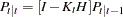 for
for  .
.
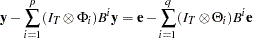
The log-likelihood function can be expressed as
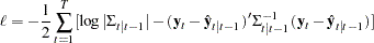 |
where  and
and  are determined recursively from the Kalman filter procedure. To construct the likelihood function from Kalman filtering, you obtain
  ,
, 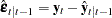 , and
, and 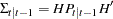 .
.
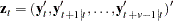
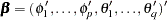
Define the vector 
 |
where  and
and  .
.
The log-likelihood equations are solved by iterative numerical procedures such as the quasi-Newton optimization. The starting values for the AR and MA parameters are obtained from the least squares estimates.
Asymptotic Distribution of the Parameter Estimates
Under the assumptions of stationarity and invertibility for the VARMA model and the assumption that is a white noise process,  is a consistent estimator for
  and
and  converges in distribution to the multivariate normal
  as
as  , where
  is the asymptotic information matrix of .
Asymptotic Distributions of Impulse Response Functions
Defining the vector
 |
the asymptotic distribution of the impulse response function for a VARMA() model is
 |
where  is the covariance matrix of the parameter estimates and
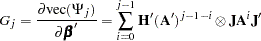 |
where 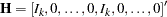 is a
is a  matrix with the second
  following after block matrices;
  is a
is a  matrix;
  is a
is a  matrix,
 |
where
 |
 is a
is a  zero matrix, and
 |
An Example of a VARMA(1,1) Model
Consider a VARMA(1,1) model with mean zero
 |
where  is the white noise process with a mean zero vector and the positive-definite covariance matrix .
The following IML procedure statements simulate a bivariate vector time series from this model to provide test data for the VARMAX procedure:
   proc iml;
      sig = {1.0  0.5, 0.5 1.25};
      phi = {1.2 -0.5, 0.6 0.3};
      theta = {0.5 -0.2, 0.1 0.3};
      /* to simulate the vector time series */
      call varmasim(y,phi,theta) sigma=sig n=100 seed=34657;
      cn = {'y1' 'y2'};
      create simul3 from y[colname=cn];
      append from y;
   run;
The following statements fit a VARMA(1,1) model to the simulated data. You specify the order of the autoregressive model with the P= option and the order of moving-average model with the Q= option. You specify the quasi-Newton optimization in the NLOPTIONS statement as an optimization method.
   proc varmax data=simul3;
      nloptions tech=qn;
      model y1 y2 / p=1 q=1 noint print=(estimates);
   run;
Figure 30.46 shows the initial values of parameters. The initial values were estimated using the least squares method.
| Optimization Start | |||
|---|---|---|---|
| Parameter Estimates | |||
| N | Parameter | Estimate | Gradient Objective Function |
| 1 | AR1_1_1 | 1.013118 | -0.987110 |
| 2 | AR1_2_1 | 0.510233 | 0.163904 |
| 3 | AR1_1_2 | -0.399051 | 0.826824 |
| 4 | AR1_2_2 | 0.441344 | -9.605845 |
| 5 | MA1_1_1 | 0.295872 | -1.929771 |
| 6 | MA1_2_1 | -0.002809 | 2.408518 |
| 7 | MA1_1_2 | -0.044216 | -0.632995 |
| 8 | MA1_2_2 | 0.425334 | 0.888222 |
Figure 30.47 shows the default option settings for the quasi-Newton optimization technique.
| Minimum Iterations | 0 |
|---|---|
| Maximum Iterations | 200 |
| Maximum Function Calls | 2000 |
| ABSGCONV Gradient Criterion | 0.00001 |
| GCONV Gradient Criterion | 1E-8 |
| ABSFCONV Function Criterion | 0 |
| FCONV Function Criterion | 2.220446E-16 |
| FCONV2 Function Criterion | 0 |
| FSIZE Parameter | 0 |
| ABSXCONV Parameter Change Criterion | 0 |
| XCONV Parameter Change Criterion | 0 |
| XSIZE Parameter | 0 |
| ABSCONV Function Criterion | -1.34078E154 |
| Line Search Method | 2 |
| Starting Alpha for Line Search | 1 |
| Line Search Precision LSPRECISION | 0.4 |
| DAMPSTEP Parameter for Line Search | . |
| Singularity Tolerance (SINGULAR) | 1E-8 |
Figure 30.48 shows the iteration history of parameter estimates.
| Iteration | Restarts | Function Calls |
Active Constraints |
Objective Function |
Objective Function Change |
Max Abs Gradient Element |
Step Size |
Slope of Search Direction |
||
|---|---|---|---|---|---|---|---|---|---|---|
| 1 | 0 | 38 | 0 | 121.86537 | 0.1020 | 6.3068 | 0.00376 | -54.483 | ||
| 2 | 0 | 57 | 0 | 121.76369 | 0.1017 | 6.9381 | 0.0100 | -33.359 | ||
| 3 | 0 | 76 | 0 | 121.55605 | 0.2076 | 5.1526 | 0.0100 | -31.265 | ||
| 4 | 0 | 95 | 0 | 121.36386 | 0.1922 | 5.7292 | 0.0100 | -37.419 | ||
| 5 | 0 | 114 | 0 | 121.25741 | 0.1064 | 5.5107 | 0.0100 | -17.708 | ||
| 6 | 0 | 133 | 0 | 121.22578 | 0.0316 | 4.9213 | 0.0240 | -2.905 | ||
| 7 | 0 | 152 | 0 | 121.20582 | 0.0200 | 6.0114 | 0.0316 | -1.268 | ||
| 8 | 0 | 171 | 0 | 121.18747 | 0.0183 | 5.5324 | 0.0457 | -0.805 | ||
| 9 | 0 | 207 | 0 | 121.13613 | 0.0513 | 0.5829 | 0.628 | -0.164 | ||
| 10 | 0 | 226 | 0 | 121.13536 | 0.000766 | 0.2054 | 1.000 | -0.0021 | ||
| 11 | 0 | 245 | 0 | 121.13528 | 0.000082 | 0.0534 | 1.000 | -0.0002 | ||
| 12 | 0 | 264 | 0 | 121.13528 | 2.537E-6 | 0.0101 | 1.000 | -637E-8 | ||
| 13 | 0 | 283 | 0 | 121.13528 | 1.475E-7 | 0.000270 | 1.000 | -3E-7 |
Figure 30.49 shows the final parameter estimates.
| Optimization Results | ||
|---|---|---|
| Parameter Estimates | ||
| N | Parameter | Estimate |
| 1 | AR1_1_1 | 1.018085 |
| 2 | AR1_2_1 | 0.391465 |
| 3 | AR1_1_2 | -0.386513 |
| 4 | AR1_2_2 | 0.552904 |
| 5 | MA1_1_1 | 0.322906 |
| 6 | MA1_2_1 | -0.165661 |
| 7 | MA1_1_2 | -0.021533 |
| 8 | MA1_2_2 | 0.586132 |
Figure 30.50 shows the AR coefficient matrix in terms of lag 1, the MA coefficient matrix in terms of lag 1, the parameter estimates, and their significance, which is one indication of how well the model fits the data.
| Type of Model | VARMA(1,1) |
|---|---|
| Estimation Method | Maximum Likelihood Estimation |
| AR | |||
|---|---|---|---|
| Lag | Variable | y1 | y2 |
| 1 | y1 | 1.01809 | -0.38651 |
| y2 | 0.39147 | 0.55290 | |
| MA | |||
|---|---|---|---|
| Lag | Variable | e1 | e2 |
| 1 | y1 | 0.32291 | -0.02153 |
| y2 | -0.16566 | 0.58613 | |
| Schematic Representation | ||
|---|---|---|
| Variable/Lag | AR1 | MA1 |
| y1 | +- | +. |
| y2 | ++ | .+ |
| + is > 2*std error, - is < -2*std error, . is between, * is N/A | ||
| Model Parameter Estimates | ||||||
|---|---|---|---|---|---|---|
| Equation | Parameter | Estimate | Standard Error |
t Value | Pr > |t| | Variable |
| y1 | AR1_1_1 | 1.01809 | 0.10256 | 9.93 | 0.0001 | y1(t-1) |
| AR1_1_2 | -0.38651 | 0.09643 | -4.01 | 0.0001 | y2(t-1) | |
| MA1_1_1 | 0.32291 | 0.14529 | 2.22 | 0.0285 | e1(t-1) | |
| MA1_1_2 | -0.02153 | 0.14199 | -0.15 | 0.8798 | e2(t-1) | |
| y2 | AR1_2_1 | 0.39147 | 0.10062 | 3.89 | 0.0002 | y1(t-1) |
| AR1_2_2 | 0.55290 | 0.08421 | 6.57 | 0.0001 | y2(t-1) | |
| MA1_2_1 | -0.16566 | 0.15699 | -1.06 | 0.2939 | e1(t-1) | |
| MA1_2_2 | 0.58612 | 0.14114 | 4.15 | 0.0001 | e2(t-1) | |
The fitted VARMA(1,1) model with estimated standard errors in parentheses is given as
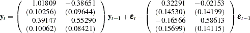 |
VARMAX Modeling
A VARMAX( ) process is written as
 |
or
 |
where ,  , and .
The dimension of the state-space vector of the Kalman filtering method for the parameter estimation of the VARMAX(,, ) model is large, which takes time and memory for computing. For convenience, the parameter estimation of the VARMAX(,,) model uses the two-stage estimation method, which first estimates the deterministic terms and exogenous parameters, and then maximizes the log-likelihood function of a VARMA(,) model.
Some examples of VARMAX modeling are as follows:
   model y1 y2 = x1 / q=1;
   nloptions tech=qn;
   model y1 y2 = x1 / p=1 q=1 xlag=1 nocurrentx;
   nloptions tech=qn;
Copyright © 2008 by SAS Institute Inc., Cary, NC, USA. All rights reserved.