| The VARMAX Procedure |
| VAR and VARX Modeling |
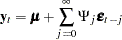
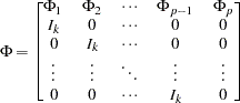
The  th-order VAR process is written as
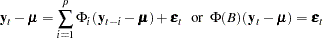 |
with 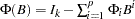 .
.
Equivalently, it can be written as
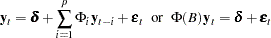 |
with 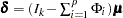 .
.
Stationarity
For stationarity, the VAR process must be expressible in the convergent causal infinite MA form as
 |
where 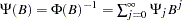 with
with  , where
  denotes a norm for the matrix
  such as
  . The matrix
  can be recursively obtained from the relation
  ; it is
 |
where  and
and  for
for  .
.
The stationarity condition is satisfied if all roots of  are outside of the unit circle. The stationarity condition is equivalent to the condition in the corresponding VAR(1) representation,
 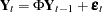 , that all eigenvalues of the
  companion matrix
  be less than one in absolute value, where
 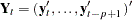 ,
, 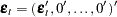 , and
, and
 |
If the stationarity condition is not satisfied, a nonstationary model (a differenced model or an error correction model) might be more appropriate.
The following statements estimate a VAR(1) model and use the ROOTS option to compute the characteristic polynomial roots:
   proc varmax data=simul1;
      model y1 y2 / p=1 noint print=(roots);
   run;
Figure 30.44 shows the output associated with the ROOTS option, which indicates that the series is stationary since the modulus of the eigenvalue is less than one.
| Roots of AR Characteristic Polynomial | |||||
|---|---|---|---|---|---|
| Index | Real | Imaginary | Modulus | Radian | Degree |
| 1 | 0.77238 | 0.35899 | 0.8517 | 0.4351 | 24.9284 |
| 2 | 0.77238 | -0.35899 | 0.8517 | -0.4351 | -24.9284 |
Parameter Estimation
Consider the stationary VAR() model
 |
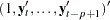
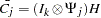
where  are assumed to be available (for convenience of notation). This can be represented by the general form of the multivariate linear model,
 |
where
 |
 |
 |
|||
 |
|
 |
|||
 |
|
 |
|||
 |
|
 |
|||
 |
|
 |
|||
 |
|
 |
|||
 |
|
 |
|||
 |
|
 |
with vec denoting the column stacking operator.
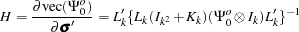
The conditional least squares estimator of  is
is
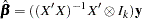 |
and the estimate of  is
is
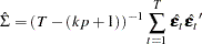 |
where  is the residual vectors. Consistency and asymptotic normality of the LS estimator are that
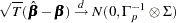 |
where  converges in probability to
  and
and  denotes convergence in distribution.
The (conditional) maximum likelihood estimator in the VAR() model is equal to the (conditional) least squares estimator on the assumption of normality of the error vectors.
Asymptotic Distributions of Impulse Response Functions
As before, vec denotes the column stacking operator and vech is the corresponding operator that stacks the elements on and below the diagonal. For any  matrix , the commutation matrix
  is defined as
 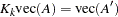 ; the duplication matrix
  is defined as
 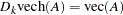 ; the elimination matrix
  is defined as
 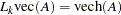 .
.
The asymptotic distribution of the impulse response function (Lütkepohl 1993) is
 |
where  and
and
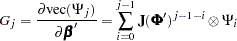 |
where  is a
is a  matrix and
  is a
is a  companion matrix.
The asymptotic distribution of the accumulated impulse response function is
 |
where  .
.
The asymptotic distribution of the orthogonalized impulse response function is
 |
where  ,
, 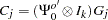 ,
,  ,
,
 |
and 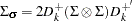 with
with 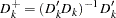 and
and  .
.
Granger Causality Test
Let  be arranged and partitioned in subgroups
  and
and  with dimensions
  and
and  , respectively (
 ); that is,
  with the corresponding white noise process
  . Consider the VAR() model with partitioned coefficients
  for
for  as follows:
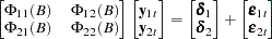 |
The variables are said to cause , but do not cause if  . The implication of this model structure is that future values of the process are influenced only by its own past and not by the past of , where future values of are influenced by the past of both and . If the future are not influenced by the past values of , then it can be better to model separately from .
Consider testing  , where
  is a
is a  matrix of rank
  and
and  is an -dimensional vector where
  . Assuming that
|
you get the Wald statistic
 |
For the Granger causality test, the matrix consists of zeros or ones and is the zero vector. See Lütkepohl(1993) for more details of the Granger causality test.
VARX Modeling
The vector autoregressive model with exogenous variables is called the VARX(,) model. The form of the VARX(,) model can be written as
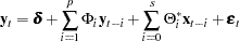 |
The parameter estimates can be obtained by representing the general form of the multivariate linear model,
|
where
|
|
|
|||
|
|
 |
|||
|
|
|
|||
|
|
 |
|||
|
|
|
|||
|
|
|
|||
|
|
|
|||
|
|
|
The conditional least squares estimator of  can be obtained by using the same method in a VAR() modeling. If the multivariate linear model has different independent variables that correspond to dependent variables, the SUR (seemingly unrelated regression) method is used to improve the regression estimates.
The following example fits the ordinary regression model:
   proc varmax data=one;
      model y1-y3 = x1-x5;
   run;
This is equivalent to the REG procedure in the SAS/STAT software:
   proc reg data=one;
      model y1 = x1-x5;
      model y2 = x1-x5;
      model y3 = x1-x5;
   run;
The following example fits the second-order lagged regression model:
   proc varmax data=two;
      model y1 y2 = x / xlag=2;
   run;
This is equivalent to the REG procedure in the SAS/STAT software:
   data three;
      set two;
      xlag1 = lag1(x);
      xlag2 = lag2(x);
   run;

   proc reg data=three;
      model y1 = x xlag1 xlag2;
      model y2 = x xlag1 xlag2;
   run;
The following example fits the ordinary regression model with different regressors:
   proc varmax data=one;
      model y1 = x1-x3, y2 = x2 x3;
   run;
This is equivalent to the following SYSLIN procedure statements:
   proc syslin data=one vardef=df sur;
      endogenous y1 y2;
      model y1 = x1-x3;
      model y2 = x2 x3;
   run;
From the output in Figure 30.20 in the section Getting Started: VARMAX Procedure, you can see that the parameters, XL0_1_2, XL0_2_1, XL0_3_1, and XL0_3_2 associated with the exogenous variables, are not significant. The following example fits the VARX(1,0) model with different regressors:
   proc varmax data=grunfeld;
      model y1 = x1, y2 = x2, y3 / p=1 print=(estimates);
   run;
| XLag | |||
|---|---|---|---|
| Lag | Variable | x1 | x2 |
| 0 | y1 | 1.83231 | _ |
| y2 | _ | 2.42110 | |
| y3 | _ | _ | |
As you can see in Figure 30.45, the symbol ‘_’ in the elements of matrix corresponds to endogenous variables that do not take the denoted exogenous variables.
Copyright © 2008 by SAS Institute Inc., Cary, NC, USA. All rights reserved.