Time Trend Curves

From the Develop Models window, select Fit ARIMA Model. From the ARIMA Model Specification window, select Add and then select Trend Curve from the menu (shown in Figure 41.1). A menu of different kinds of trend curves is displayed, as shown in Figure 41.5.

Figure 41.5 Time Trend Curves Menu

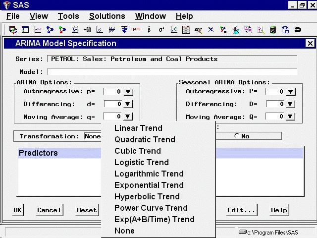
These trend curves work in a similar way as the Linear Trend option (which is a special case of a trend curve and one of the choices on the menu), but with the Trend Curve menu you have a choice of various nonlinear time trends.

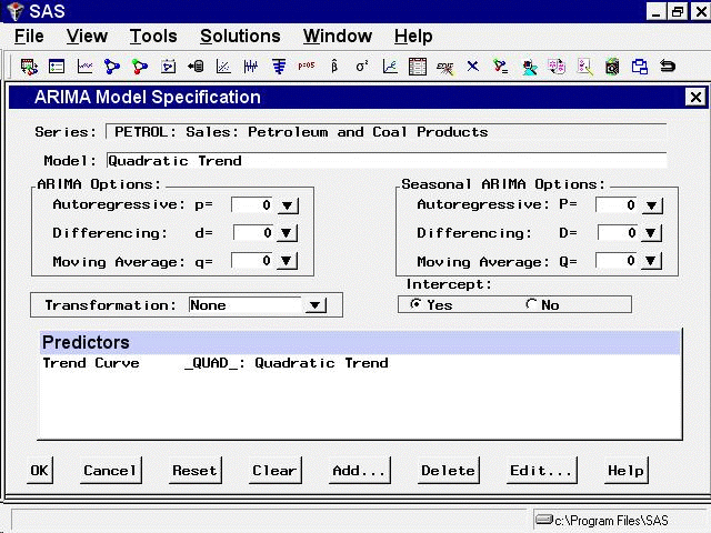
Select Quadratic Trend. This adds a quadratic time trend to the Predictors list, as shown in Figure 41.6.

Figure 41.6 Quadratic Trend Specified

Now select the OK button. The quadratic trend model is fit and added to the list of models in the Develop Models window. The Model Viewer displays a plot of the quadratic trend model, as shown in Figure 41.7.

Figure 41.7 Quadratic Trend Model

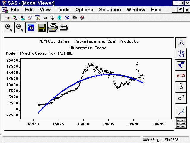
This curve does not fit the PETROL series very well, but the View Model plot illustrates how time trend models work. You might want to experiment with different trend models to see what the different trend curves look like.

Some of the trend curves require transforming the dependent series. When you specify one of these curves, a notice is displayed reminding you that a transformation is needed, and the Transformation field is automatically filled in. Therefore, you cannot control the Transformation specification when some kinds of trend curves are specified.

See the section Time Trend Curves in Chapter 44, Forecasting Process Details, for more information about the different trend curves.