| The SYSLIN Procedure |
Example 26.3 Illustration of ODS Graphics
This example illustrates the use of ODS graphics. This is a continuation of the section Klein’s Model I Estimated with LIML and 3SLS. These graphical displays are requested by specifying the ODS GRAPHICS statement before running PROC SYSLIN. For information about the graphics available in the SYSLIN procedure, see the section ODS Graphics.
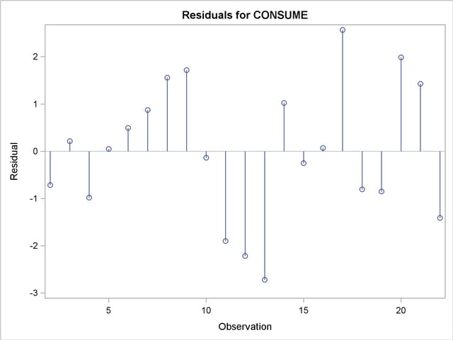
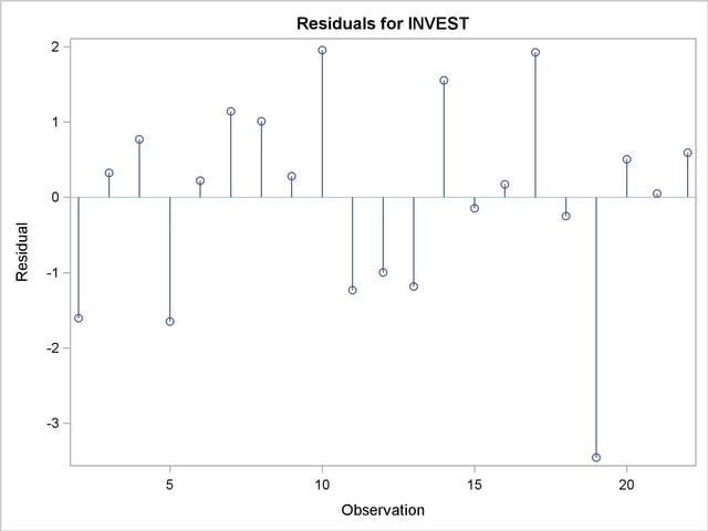
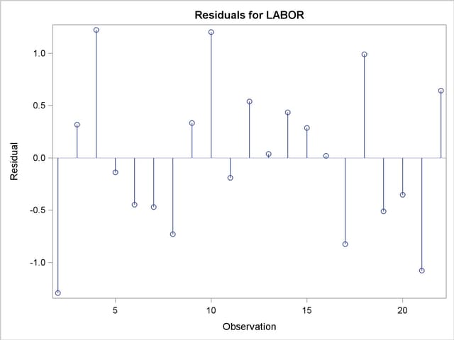
The following statements show how to generate ODS graphics plots with the SYSLIN procedure. The plots of residuals for each one of the equations in the model are displayed in Figure 26.3.1 through Figure 26.3.3.
   *---------------------------Klein's Model I----------------------------*
   | By L.R. Klein, Economic Fluctuations in the United States, 1921-1941 |
   | (1950), NY: John Wiley.   A macro-economic model of the U.S. with    |
   | three behavioral equations, and several identities. See Theil, p.456.|
   *----------------------------------------------------------------------*;
   data klein;
   input year c p w i x wp g t k wsum;
      date=mdy(1,1,year);
      format date monyy.;
      y   =c+i+g-t;
      yr  =year-1931;
      klag=lag(k);
      plag=lag(p);
      xlag=lag(x);
      label year='Year'
            date='Date'
            c   ='Consumption'
            p   ='Profits'
            w   ='Private Wage Bill'
            i   ='Investment'
            k   ='Capital Stock'
            y   ='National Income'
            x   ='Private Production'
            wsum='Total Wage Bill'
            wp  ='Govt Wage Bill'
            g   ='Govt Demand'
            i   ='Taxes'
            klag='Capital Stock Lagged'
            plag='Profits Lagged'
            xlag='Private Product Lagged'
            yr  ='YEAR-1931';
   datalines;
   1920     .  12.7     .    .  44.9    .     .     .  182.8     .
   1921  41.9  12.4  25.5 -0.2  45.6  2.7   3.9   7.7  182.6  28.2
   1922  45.0  16.9  29.3  1.9  50.1  2.9   3.2   3.9  184.5  32.2
   1923  49.2  18.4  34.1  5.2  57.2  2.9   2.8   4.7  189.7  37.0
   1924  50.6  19.4  33.9  3.0  57.1  3.1   3.5   3.8  192.7  37.0
   1925  52.6  20.1  35.4  5.1  61.0  3.2   3.3   5.5  197.8  38.6
   1926  55.1  19.6  37.4  5.6  64.0  3.3   3.3   7.0  203.4  40.7
   1927  56.2  19.8  37.9  4.2  64.4  3.6   4.0   6.7  207.6  41.5
   1928  57.3  21.1  39.2  3.0  64.5  3.7   4.2   4.2  210.6  42.9
   1929  57.8  21.7  41.3  5.1  67.0  4.0   4.1   4.0  215.7  45.3

   ... more lines ...
   ods graphics on;

   proc syslin data=klein outest=b liml plots(unpack only)=residual ;
      endogenous c p w i x wsum k y;
      instruments klag plag xlag wp g t yr;
      consume: model c = p plag  wsum;
      invest:  model i = p plag  klag;
      labor:   model w = x xlag  yr;
   run;
Output 26.3.1
Residuals Diagnostic Plots for Consumption
Output 26.3.2
Residuals Diagnostic Plots for Investments
Output 26.3.3
Residuals Diagnostic Plots for Labor
Copyright © 2008 by SAS Institute Inc., Cary, NC, USA. All rights reserved.