PROC SIMLIN: Simulating Klein’s Model I :: SAS/ETS(R) 9.2 User's Guide

The SIMLIN Procedure

Example 23.1 Simulating Klein’s Model I

In this example, the SIMLIN procedure simulates a model of the U.S. economy called Klein’s Model I. The SAS data set KLEIN is used as input to the SYSLIN and SIMLIN procedures.

   data klein;
      input year c p w i x wp g t k wsum;
      date=mdy(1,1,year);
      format date year.;
      y   = c + i + g - t;
      yr  = year - 1931;
      klag = lag( k );
      plag = lag( p );
      xlag = lag( x );
      if year >= 1921;
      label c   ='consumption'
            p   ='profits'
            w   ='private wage bill'
            i   ='investment'
            k   ='capital stock'
            y   ='national income'
            x   ='private production'
            wsum='total wage bill'
            wp  ='govt wage bill'
            g   ='govt demand'
            t   ='taxes'
            klag='capital stock lagged'
            plag='profits lagged'
            xlag='private product lagged'
            yr  ='year-1931';
   datalines;
   1920     .  12.7     .    .  44.9    .     .     .  182.8     .
   
   ... more lines ...

First, the model is specified and estimated using the SYSLIN procedure, and the parameter estimates are written to an OUTEST= data set. The printed output produced by the SYSLIN procedure is not shown here; see Example 26.1 in Chapter 26 for the printed output of the PROC SYSLIN step.

   title1 'Simulation of Klein''s Model I using SIMLIN';
   proc syslin 3sls data=klein outest=a;
   
      instruments klag plag xlag wp g t yr;
      endogenous c p w i x wsum k y;
   
      consume: model    c = p plag wsum;
      invest:  model    i = p plag klag;
      labor:   model    w = x xlag yr;
   
      product: identity x = c + i + g;
      income:  identity y = c + i + g - t;
      profit:  identity p = x - w - t;
      stock:   identity k = klag + i;
      wage:    identity wsum = w + wp;
   run;

The OUTEST= data set A created by the SYSLIN procedure contains parameter estimates to be used by the SIMLIN procedure. The OUTEST= data set is shown in Output 23.1.1.

Output 23.1.1 The OUTEST= Data Set Created by PROC SYSLIN

Simulation of Klein's Model I using SIMLIN

Obs	_TYPE_	_STATUS_	_MODEL_	_DEPVAR_	_SIGMA_	Intercept	klag	plag	xlag	wp	g	t	yr	c	p	w	i	x	wsum	k	y
1	INST	0 Converged	FIRST	c	2.11403	58.3018	-0.14654	0.74803	0.23007	0.19327	0.20501	-0.36573	0.70109	-1	.	.	.	.	.	.	.
2	INST	0 Converged	FIRST	p	2.18298	50.3844	-0.21610	0.80250	0.02200	-0.07961	0.43902	-0.92310	0.31941	.	-1.00000	.	.	.	.	.	.
3	INST	0 Converged	FIRST	w	1.75427	43.4356	-0.12295	0.87192	0.09533	-0.44373	0.86622	-0.60415	0.71358	.	.	-1	.	.	.	.	.
4	INST	0 Converged	FIRST	i	1.72376	35.5182	-0.19251	0.92639	-0.11274	-0.71661	0.10023	-0.16152	0.33190	.	.	.	-1	.	.	.	.
5	INST	0 Converged	FIRST	x	3.77347	93.8200	-0.33906	1.67442	0.11733	-0.52334	1.30524	-0.52725	1.03299	.	.	.	.	-1.00000	.	.	.
6	INST	0 Converged	FIRST	wsum	1.75427	43.4356	-0.12295	0.87192	0.09533	0.55627	0.86622	-0.60415	0.71358	.	.	.	.	.	-1.00000	.	.
7	INST	0 Converged	FIRST	k	1.72376	35.5182	0.80749	0.92639	-0.11274	-0.71661	0.10023	-0.16152	0.33190	.	.	.	.	.	.	-1	.
8	INST	0 Converged	FIRST	y	3.77347	93.8200	-0.33906	1.67442	0.11733	-0.52334	1.30524	-1.52725	1.03299	.	.	.	.	.	.	.	-1
9	3SLS	0 Converged	CONSUME	c	1.04956	16.4408	.	0.16314	.	.	.	.	.	-1	0.12489	.	.	.	0.79008	.	.
10	3SLS	0 Converged	INVEST	i	1.60796	28.1778	-0.19485	0.75572	.	.	.	.	.	.	-0.01308	.	-1	.	.	.	.
11	3SLS	0 Converged	LABOR	w	0.80149	1.7972	.	.	0.18129	.	.	.	0.14967	.	.	-1	.	0.40049	.	.	.
12	IDENTITY	0 Converged	PRODUCT	x	.	0.0000	.	.	.	.	1.00000	.	.	1	.	.	1	-1.00000	.	.	.
13	IDENTITY	0 Converged	INCOME	y	.	0.0000	.	.	.	.	1.00000	-1.00000	.	1	.	.	1	.	.	.	-1
14	IDENTITY	0 Converged	PROFIT	p	.	0.0000	.	.	.	.	.	-1.00000	.	.	-1.00000	-1	.	1.00000	.	.	.
15	IDENTITY	0 Converged	STOCK	k	.	0.0000	1.00000	.	.	.	.	.	.	.	.	.	1	.	.	-1	.
16	IDENTITY	0 Converged	WAGE	wsum	.	0.0000	.	.	.	1.00000	.	.	.	.	.	1	.	.	-1.00000	.	.

Using the OUTEST= data set A produced by the SYSLIN procedure, the SIMLIN procedure can now compute the reduced form and simulate the model. The following statements perform the simulation.

   title1 'Simulation of Klein''s Model I using SIMLIN';
   proc simlin data=klein 
               est=a type=3sls
               estprint 
               total interim=2 
               outest=b;
      endogenous c p w i x wsum k y;
      exogenous  wp g t yr;
      lagged  klag k 1   plag p 1   xlag x 1;
      id year;
      output out=c p=chat phat what ihat xhat wsumhat khat yhat
                   r=cres pres wres ires xres wsumres kres yres;
   run;

The reduced form coefficients and multipliers are added to the information read from EST= data set A and written to the OUTEST= data set B. The predicted and residual values from the simulation are written to the OUT= data set C specified in the OUTPUT statement.

The SIMLIN procedure first prints the structural coefficient matrices read from the EST= data set, as shown in Output 23.1.2 through Output 23.1.4.

Output 23.1.2 SIMLIN Procedure Output – Endogenous Structural Coefficients

Simulation of Klein's Model I using SIMLIN

The SIMLIN Procedure

Structural Coefficients for Endogenous Variables
Variable	c	p	w	i	x	wsum	k	y
c	1.0000	-0.1249	.	.	.	-0.7901	.	.
i	.	0.0131	.	1.0000	.	.	.	.
w	.	.	1.0000	.	-0.4005	.	.	.
x	-1.0000	.	.	-1.0000	1.0000	.	.	.
y	-1.0000	.	.	-1.0000	.	.	.	1.0000
p	.	1.0000	1.0000	.	-1.0000	.	.	.
k	.	.	.	-1.0000	.	.	1.0000	.
wsum	.	.	-1.0000	.	.	1.0000	.	.

Output 23.1.3 SIMLIN Procedure Output – Lagged Endogenous Structural Coefficients

Structural Coefficients for Lagged Endogenous Variables
Variable	klag	plag	xlag
c	.	0.1631	.
i	-0.1948	0.7557	.
w	.	.	0.1813
x	.	.	.
y	.	.	.
p	.	.	.
k	1.0000	.	.
wsum	.	.	.

Output 23.1.4 SIMLIN Procedure Output – Exogenous Structural Coefficients

Structural Coefficients for Exogenous Variables
Variable	wp	g	t	yr	Intercept
c	.	.	.	.	16.4408
i	.	.	.	.	28.1778
w	.	.	.	0.1497	1.7972
x	.	1.0000	.	.	0
y	.	1.0000	-1.0000	.	0
p	.	.	-1.0000	.	0
k	.	.	.	.	0
wsum	1.0000	.	.	.	0

The SIMLIN procedure then prints the inverse of the endogenous variables coefficient matrix, as shown in Output 23.1.5.

Output 23.1.5 SIMLIN Procedure Output – Inverse Coefficient Matrix

Inverse Coefficient Matrix for Endogenous Variables
Variable	c	i	w	x	y	p	k	wsum
c	1.6347	0.6347	1.0957	0.6347	0	0.1959	0	1.2915
p	0.9724	0.9724	-0.3405	0.9724	0	1.1087	0	0.7682
w	0.6496	0.6496	1.4406	0.6496	0	0.0726	0	0.5132
i	-0.0127	0.9873	0.004453	-0.0127	0	-0.0145	0	-0.0100
x	1.6219	1.6219	1.1001	1.6219	0	0.1814	0	1.2815
wsum	0.6496	0.6496	1.4406	0.6496	0	0.0726	0	1.5132
k	-0.0127	0.9873	0.004453	-0.0127	0	-0.0145	1.0000	-0.0100
y	1.6219	1.6219	1.1001	0.6219	1.0000	0.1814	0	1.2815

The SIMLIN procedure next prints the reduced form coefficient matrices, as shown in Output 23.1.6.

Output 23.1.6 SIMLIN Procedure Output – Reduced Form Coefficients

Reduced Form for Lagged Endogenous Variables
Variable	klag	plag	xlag
c	-0.1237	0.7463	0.1986
p	-0.1895	0.8935	-0.0617
w	-0.1266	0.5969	0.2612
i	-0.1924	0.7440	0.000807
x	-0.3160	1.4903	0.1994
wsum	-0.1266	0.5969	0.2612
k	0.8076	0.7440	0.000807
y	-0.3160	1.4903	0.1994

Reduced Form for Exogenous Variables
Variable	wp	g	t	yr	Intercept
c	1.2915	0.6347	-0.1959	0.1640	46.7273
p	0.7682	0.9724	-1.1087	-0.0510	42.7736
w	0.5132	0.6496	-0.0726	0.2156	31.5721
i	-0.0100	-0.0127	0.0145	0.000667	27.6184
x	1.2815	1.6219	-0.1814	0.1647	74.3457
wsum	1.5132	0.6496	-0.0726	0.2156	31.5721
k	-0.0100	-0.0127	0.0145	0.000667	27.6184
y	1.2815	1.6219	-1.1814	0.1647	74.3457

The multiplier matrices (requested by the INTERIM=2 and TOTAL options) are printed next, as shown in Output 23.1.7 and Output 23.1.8.

Output 23.1.7 SIMLIN Procedure Output – Interim Multipliers

Interim Multipliers for Interim 1
Variable	wp	g	t	yr	Intercept
c	0.829130	1.049424	-0.865262	-.0054080	43.27442
p	0.609213	0.771077	-0.982167	-.0558215	28.39545
w	0.794488	1.005578	-0.710961	0.0125018	41.45124
i	0.574572	0.727231	-0.827867	-.0379117	26.57227
x	1.403702	1.776655	-1.693129	-.0433197	69.84670
wsum	0.794488	1.005578	-0.710961	0.0125018	41.45124
k	0.564524	0.714514	-0.813366	-.0372452	54.19068
y	1.403702	1.776655	-1.693129	-.0433197	69.84670

Interim Multipliers for Interim 2
Variable	wp	g	t	yr	Intercept
c	0.663671	0.840004	-0.968727	-.0456589	28.36428
p	0.350716	0.443899	-0.618929	-.0401446	10.79216
w	0.658769	0.833799	-0.925467	-.0399178	28.33114
i	0.345813	0.437694	-0.575669	-.0344035	10.75901
x	1.009485	1.277698	-1.544396	-.0800624	39.12330
wsum	0.658769	0.833799	-0.925467	-.0399178	28.33114
k	0.910337	1.152208	-1.389035	-.0716486	64.94969
y	1.009485	1.277698	-1.544396	-.0800624	39.12330

Output 23.1.8 SIMLIN Procedure Output – Total Multipliers

Total Multipliers
Variable	wp	g	t	yr	Intercept
c	1.881667	1.381613	-0.685987	0.1789624	41.3045
p	0.786945	0.996031	-1.286891	-.0748290	15.4770
w	1.094722	1.385582	-0.399095	0.2537914	25.8275
i	0.000000	0.000000	-0.000000	0.0000000	0.0000
x	1.881667	2.381613	-0.685987	0.1789624	41.3045
wsum	2.094722	1.385582	-0.399095	0.2537914	25.8275
k	2.999365	3.796275	-4.904859	-.2852032	203.6035
y	1.881667	2.381613	-1.685987	0.1789624	41.3045

The last part of the SIMLIN procedure output is a table of statistics of fit for the simulation, as shown in Output 23.1.9.

Output 23.1.9 SIMLIN Procedure Output – Simulation Statistics

Fit Statistics
Variable	N	Mean Error	Mean Pct Error	Mean Abs Error	Mean Abs Pct Error	RMS Error	RMS Pct Error	Label
c	21	0.1367	-0.3827	3.5011	6.69769	4.3155	8.1701	consumption
p	21	0.1422	-4.0671	2.9355	19.61400	3.4257	26.0265	profits
w	21	0.1282	-0.8939	3.1247	8.92110	4.0930	11.4709	private wage bill
i	21	0.1337	105.8529	2.4983	127.13736	2.9980	252.3497	investment
x	21	0.2704	-0.9553	5.9622	10.40057	7.1881	12.5653	private production
wsum	21	0.1282	-0.6669	3.1247	7.88988	4.0930	10.1724	total wage bill
k	21	-0.1424	-0.1506	3.8879	1.90614	5.0036	2.4209	capital stock
y	21	0.2704	-1.3476	5.9622	11.74177	7.1881	14.2214	national income

The OUTEST= output data set contains all the observations read from the EST= data set, and in addition contains observations for the reduced form and multiplier matrices. The following statements produce a partial listing of the OUTEST= data set, as shown in Output 23.1.10.

   proc print data=b;
      where _type_ = 'REDUCED' | _type_ = 'IMULT1';
   run;

Output 23.1.10 Partial Listing of OUTEST= Data Set

Simulation of Klein's Model I using SIMLIN

Obs	_TYPE_	_DEPVAR_	_SIGMA_	c	p	w	i	x	wsum	k	y	klag	plag	xlag	wp	g	t	yr	Intercept
9	REDUCED	c	.	1.63465	0.63465	1.09566	0.63465	0	0.19585	0	1.29151	-0.12366	0.74631	0.19863	1.29151	0.63465	-0.19585	0.16399	46.7273
10	REDUCED	p	.	0.97236	0.97236	-0.34048	0.97236	0	1.10872	0	0.76825	-0.18946	0.89347	-0.06173	0.76825	0.97236	-1.10872	-0.05096	42.7736
11	REDUCED	w	.	0.64957	0.64957	1.44059	0.64957	0	0.07263	0	0.51321	-0.12657	0.59687	0.26117	0.51321	0.64957	-0.07263	0.21562	31.5721
12	REDUCED	i	.	-0.01272	0.98728	0.00445	-0.01272	0	-0.01450	0	-0.01005	-0.19237	0.74404	0.00081	-0.01005	-0.01272	0.01450	0.00067	27.6184
13	REDUCED	x	.	1.62194	1.62194	1.10011	1.62194	0	0.18135	0	1.28146	-0.31603	1.49034	0.19944	1.28146	1.62194	-0.18135	0.16466	74.3457
14	REDUCED	wsum	.	0.64957	0.64957	1.44059	0.64957	0	0.07263	0	1.51321	-0.12657	0.59687	0.26117	1.51321	0.64957	-0.07263	0.21562	31.5721
15	REDUCED	k	.	-0.01272	0.98728	0.00445	-0.01272	0	-0.01450	1	-0.01005	0.80763	0.74404	0.00081	-0.01005	-0.01272	0.01450	0.00067	27.6184
16	REDUCED	y	.	1.62194	1.62194	1.10011	0.62194	1	0.18135	0	1.28146	-0.31603	1.49034	0.19944	1.28146	1.62194	-1.18135	0.16466	74.3457
17	IMULT1	c	.	.	.	.	.	.	.	.	.	.	.	.	0.82913	1.04942	-0.86526	-0.00541	43.2744
18	IMULT1	p	.	.	.	.	.	.	.	.	.	.	.	.	0.60921	0.77108	-0.98217	-0.05582	28.3955
19	IMULT1	w	.	.	.	.	.	.	.	.	.	.	.	.	0.79449	1.00558	-0.71096	0.01250	41.4512
20	IMULT1	i	.	.	.	.	.	.	.	.	.	.	.	.	0.57457	0.72723	-0.82787	-0.03791	26.5723
21	IMULT1	x	.	.	.	.	.	.	.	.	.	.	.	.	1.40370	1.77666	-1.69313	-0.04332	69.8467
22	IMULT1	wsum	.	.	.	.	.	.	.	.	.	.	.	.	0.79449	1.00558	-0.71096	0.01250	41.4512
23	IMULT1	k	.	.	.	.	.	.	.	.	.	.	.	.	0.56452	0.71451	-0.81337	-0.03725	54.1907
24	IMULT1	y	.	.	.	.	.	.	.	.	.	.	.	.	1.40370	1.77666	-1.69313	-0.04332	69.8467

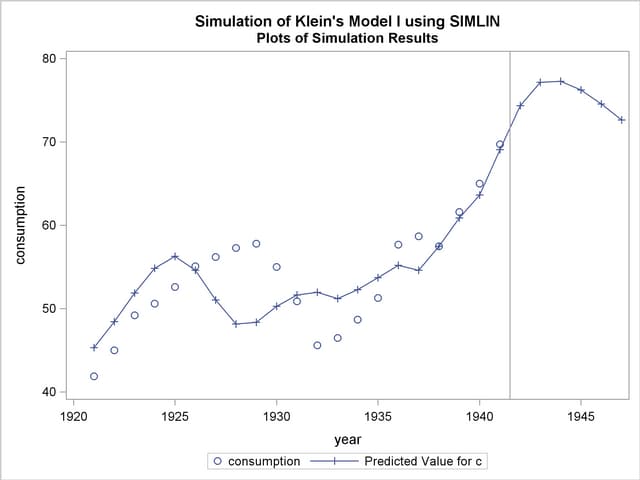
The actual and predicted values for the variable C are plotted in Output 23.1.11.

   title2 'Plots of Simulation Results';
   proc sgplot data=c;
      scatter x=year y=c;
      series x=year y=chat / markers markerattrs=(symbol=plus);
      refline 1941.5 / axis=x;
   run;

Output 23.1.11 Plot of Actual and Predicted Consumption

Top of Page