PROC MODEL: Polynomial Distributed Lags by Using %PDL

The MODEL Procedure

Example 18.5 Polynomial Distributed Lags by Using %PDL

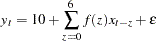
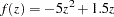
This example shows the use of the %PDL macro for polynomial distributed lag models. Simulated data is generated so that Y is a linear function of six lags of X, with the lag coefficients following a quadratic polynomial. The model is estimated by using a fourth-degree polynomial, both with and without endpoint constraints. The example uses simulated data generated from the following model:

$\text{[math]}$

The LIST option prints the model statements added by the %PDL macro. The following statements generate simulated data as shown:

   /*--------------------------------------------------------------*/
   /*  Generate Simulated Data for a Linear Model with a PDL on X  */
   /*        y = 10 + x(6,2) + e                                   */
   /*        pdl(x) = -5.*(lg)**2 + 1.5*(lg) + 0.                  */
   /*--------------------------------------------------------------*/
   data pdl;
      pdl2=-5.; pdl1=1.5; pdl0=0;
      array zz(i) z0-z6;
      do i=1 to 7;
         z=i-1;
         zz=pdl2*z**2 + pdl1*z + pdl0;
         end;
      do n=-11 to 30;
         x  =10*ranuni(1234567)-5;
         pdl=z0*x + z1*xl1 + z2*xl2 + z3*xl3 + z4*xl4 + z5*xl5 + z6*xl6;
         e  =10*rannor(123);
         y  =10+pdl+e;
         if n>=1 then output;
         xl6=xl5; xl5=xl4; xl4=xl3; xl3=xl2; xl2=xl1; xl1=x;
         end;
   run;

   title1 'Polynomial Distributed Lag Example';
   title3 'Estimation of PDL(6,4) Model-- No Endpoint Restrictions';
   
   proc model data=pdl;
      parms int;                  /* declare the intercept parameter */
      %pdl( xpdl, 6, 4 )          /* declare the lag distribution */
      y = int + %pdl( xpdl, x );  /* define the model equation */
      fit y / list;               /* estimate the parameters */
   run;

The LIST output for the model without endpoint restrictions is shown in Output 18.5.1. The first seven statements in the generated program are the polynomial expressions for lag parameters XPDL_L0 through XPDL_L6. The estimated parameters are INT, XPDL_0, XPDL_1, XPDL_2, XPDL_3, and XPDL_4.

Output 18.5.1 PROC MODEL Listing of Generated Program

Polynomial Distributed Lag Example

Estimation of PDL(6,4) Model-- No Endpoint Restrictions

The MODEL Procedure

Listing of Compiled Program Code
Stmt	Line:Col	Statement as Parsed
1	4152:14	XPDL_L0 = XPDL_0;
2	4152:14	XPDL_L1 = XPDL_0 + XPDL_1 + XPDL_2 + XPDL_3 + XPDL_4;
3	4152:14	XPDL_L2 = XPDL_0 + XPDL_1 * 2 + XPDL_2 * 2 ** 2 + XPDL_3 * 2 ** 3 + XPDL_4 * 2 ** 4;
4	4152:14	XPDL_L3 = XPDL_0 + XPDL_1 * 3 + XPDL_2 * 3 ** 2 + XPDL_3 * 3 ** 3 + XPDL_4 * 3 ** 4;
5	4152:14	XPDL_L4 = XPDL_0 + XPDL_1 * 4 + XPDL_2 * 4 ** 2 + XPDL_3 * 4 ** 3 + XPDL_4 * 4 ** 4;
6	4152:14	XPDL_L5 = XPDL_0 + XPDL_1 * 5 + XPDL_2 * 5 ** 2 + XPDL_3 * 5 ** 3 + XPDL_4 * 5 ** 4;
7	4152:14	XPDL_L6 = XPDL_0 + XPDL_1 * 6 + XPDL_2 * 6 ** 2 + XPDL_3 * 6 ** 3 + XPDL_4 * 6 ** 4;
8	4153:4	PRED.y = int + XPDL_L0 * x + XPDL_L1 * LAG1( x ) + XPDL_L2 * LAG2( x ) + XPDL_L3 * LAG3( x ) + XPDL_L4 * LAG4( x ) + XPDL_L5 * LAG5( x ) + XPDL_L6 * LAG6( x );
8	4153:4	RESID.y = PRED.y - ACTUAL.y;
8	4153:4	ERROR.y = PRED.y - y;
9	4152:15	ESTIMATE XPDL_L0, XPDL_L1, XPDL_L2, XPDL_L3, XPDL_L4, XPDL_L5, XPDL_L6;
10	4152:15	_est0 = XPDL_L0;
11	4152:15	_est1 = XPDL_L1;
12	4152:15	_est2 = XPDL_L2;
13	4152:15	_est3 = XPDL_L3;
14	4152:15	_est4 = XPDL_L4;
15	4152:15	_est5 = XPDL_L5;
16	4152:14	_est6 = XPDL_L6;

The FIT results for the model without endpoint restrictions are shown in Output 18.5.2.

Output 18.5.2 PROC MODEL Results That Specify No Endpoint Restrictions

Polynomial Distributed Lag Example

Estimation of PDL(6,4) Model-- No Endpoint Restrictions

The MODEL Procedure

Nonlinear OLS Summary of Residual Errors
Equation	DF Model	DF Error	SSE	MSE	Root MSE	R-Square	Adj R-Sq
y	6	18	2070.8	115.0	10.7259	0.9998	0.9998

Nonlinear OLS Parameter Estimates
Parameter	Estimate	Approx Std Err	t Value	Approx Pr > \|t\|	Label
int	9.621969	2.3238	4.14	0.0006
XPDL_0	0.084374	0.7587	0.11	0.9127	PDL(XPDL,6,4) parameter for (L)**0
XPDL_1	0.749956	2.0936	0.36	0.7244	PDL(XPDL,6,4) parameter for (L)**1
XPDL_2	-4.196	1.6215	-2.59	0.0186	PDL(XPDL,6,4) parameter for (L)**2
XPDL_3	-0.21489	0.4253	-0.51	0.6195	PDL(XPDL,6,4) parameter for (L)**3
XPDL_4	0.016133	0.0353	0.46	0.6528	PDL(XPDL,6,4) parameter for (L)**4

Portions of the output produced by the following PDL model with endpoints of the model restricted to zero are presented in Output 18.5.3.

   title3 'Estimation of PDL(6,4) Model-- Both Endpoint Restrictions';
   
   proc model data=pdl ;
      parms int;                  /* declare the intercept parameter */
      %pdl( xpdl, 6, 4, r=both )  /* declare the lag distribution */
      y = int + %pdl( xpdl, x );  /* define the model equation */
      fit y /list;                /* estimate the parameters */
   run;

Output 18.5.3 PROC MODEL Results Specifying Both Endpoint Restrictions

Polynomial Distributed Lag Example

Estimation of PDL(6,4) Model-- Both Endpoint Restrictions

The MODEL Procedure

Nonlinear OLS Summary of Residual Errors
Equation	DF Model	DF Error	SSE	MSE	Root MSE	R-Square	Adj R-Sq
y	4	20	449868	22493.4	150.0	0.9596	0.9535

Nonlinear OLS Parameter Estimates
Parameter	Estimate	Approx Std Err	t Value	Approx Pr > \|t\|	Label
int	17.08581	32.4032	0.53	0.6038
XPDL_2	13.88433	5.4361	2.55	0.0189	PDL(XPDL,6,4) parameter for (L)**2
XPDL_3	-9.3535	1.7602	-5.31	<.0001	PDL(XPDL,6,4) parameter for (L)**3
XPDL_4	1.032421	0.1471	7.02	<.0001	PDL(XPDL,6,4) parameter for (L)**4

Note that XPDL_0 and XPDL_1 are not shown in the estimate summary. They were used to satisfy the endpoint restrictions analytically by the generated %PDL macro code. Their values can be determined by back substitution.

To estimate the PDL model with one or more of the polynomial terms dropped, specify the largest degree of the polynomial desired with the %PDL macro and use the DROP= option in the FIT statement to remove the unwanted terms. The dropped parameters should be set to 0. The following PROC MODEL statements demonstrate estimation with a PDL of degree 2 without the 0th order term.

   title3 'Estimation of PDL(6,2) Model-- With XPDL_0 Dropped';
   
   proc model data=pdl list;
      parms int;                  /* declare the intercept parameter */
      %pdl( xpdl, 6, 2 )          /* declare the lag distribution */
      y = int + %pdl( xpdl, x );  /* define the model equation */
      xpdl_0 =0;
      fit y drop=xpdl_0;          /* estimate the parameters */
   run;

The results from this estimation are shown in Output 18.5.4.

Output 18.5.4 PROC MODEL Results That Specify %PDL( XPDL, 6, 2)

Polynomial Distributed Lag Example

Estimation of PDL(6,2) Model-- With XPDL_0 Dropped

The MODEL Procedure

Nonlinear OLS Summary of Residual Errors
Equation	DF Model	DF Error	SSE	MSE	Root MSE	R-Square	Adj R-Sq
y	3	21	2114.1	100.7	10.0335	0.9998	0.9998

Nonlinear OLS Parameter Estimates
Parameter	Estimate	Approx Std Err	t Value	Approx Pr > \|t\|	Label
int	9.536382	2.1685	4.40	0.0003
XPDL_1	1.883315	0.3159	5.96	<.0001	PDL(XPDL,6,2) parameter for (L)**1
XPDL_2	-5.08827	0.0656	-77.56	<.0001	PDL(XPDL,6,2) parameter for (L)**2

Top of Page