| The MDC Procedure |
Example 17.1 Binary Data Modeling
The MDC procedure supports various multinomial choice models. However, binary choice models such as binary logit and probit can also be estimated using PROC MDC since these models are special cases of multinomial models.
Spector and Mazzeo (1980) studied the effectiveness of a new teaching method on students’ performance in an economics course. They reported grade point average (gpa ), previous knowledge of the material (tuce ), a dummy variable for the new teaching method (psi ), and the final course grade (grade ). grade is recorded as 1 if a student earned the letter grade "A," and 0 otherwise.
The binary logit can be estimated using the conditional logit model. In order to use the MDC procedure, the data are converted as follows so that each possible choice corresponds to one observation:
   data smdata;
      input gpa tuce psi grade;
   datalines;
   2.66      20      0        0
   2.89      22      0        0
   3.28      24      0        0

   ... more lines ...
   data smdata1;
      set smdata;
      retain id 0;
      id + 1;

      /*-- first choice --*/
      choice1 = 1;
      choice2 = 0;
      decision = (grade = 0);
      gpa_2 = 0;
      tuce_2 = 0;
      psi_2 = 0;
      output;

      /*-- second choice --*/
      choice1 = 0;
      choice2 = 1;
      decision = (grade = 1);
      gpa_2 = gpa;
      tuce_2 = tuce;
      psi_2 = psi;
      output;
   run;
The first 10 observations are displayed in Output 17.1.1. The variables related to grade =0 are omitted since these are not used for binary choice model estimation.
Consider the choice probability of the conditional logit model for binary choice:
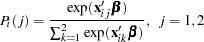 |
The choice probability of the binary logit model is computed based on normalization. The preceding conditional logit model can be converted as
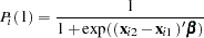 |
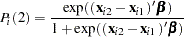 |
Therefore, you can interpret the binary choice data as the difference between the first and second choice characteristics. In the following statements, it is assumed that  . The binary logit model is estimated and displayed in Output 17.1.2.
   /*-- Conditional Logit --*/
   proc mdc data=smdata1;
      model decision = choice2 gpa_2 tuce_2 psi_2 /
               type=clogit
               nchoice=2
               covest=hess;
      id id;
   run;
| Parameter Estimates | |||||
|---|---|---|---|---|---|
| Parameter | DF | Estimate | Standard Error |
t Value | Approx Pr > |t| |
| choice2 | 1 | -13.0213 | 4.9313 | -2.64 | 0.0083 |
| gpa_2 | 1 | 2.8261 | 1.2629 | 2.24 | 0.0252 |
| tuce_2 | 1 | 0.0952 | 0.1416 | 0.67 | 0.5014 |
| psi_2 | 1 | 2.3787 | 1.0646 | 2.23 | 0.0255 |
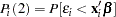
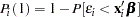
Consider the choice probability of the multinomial probit model:
 |
The probabilities of choice of the two alternatives can be written as
 |
 |
where 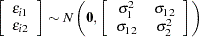 . Assume that
  and
and  . The binary probit model is estimated and displayed in Output 17.1.3. You do not get the same estimates as that of the usual binary probit model. The probabilities of choice in the binary probit model are
 |
 |
where  . However, the multinomial probit model has the error variance
  if
if  and
and  are independent (). In the following statements, unit variance restrictions are imposed on choices 1 and 2 (
 ). Therefore, the usual binary probit estimates (and standard errors) can be obtained by multiplying the multinomial probit estimates (and standard errors) in Output 17.1.3 by
  .
.
   /*-- Multinomial Probit --*/
   proc mdc data=smdata1;
      model decision = choice2 gpa_2 tuce_2 psi_2 /
               type=mprobit
               nchoice=2
               covest=hess
               unitvariance=(1 2);
      id id;
   run;
| Parameter Estimates | |||||
|---|---|---|---|---|---|
| Parameter | DF | Estimate | Standard Error |
t Value | Approx Pr > |t| |
| choice2 | 1 | -10.5392 | 3.5956 | -2.93 | 0.0034 |
| gpa_2 | 1 | 2.2992 | 0.9813 | 2.34 | 0.0191 |
| tuce_2 | 1 | 0.0732 | 0.1186 | 0.62 | 0.5375 |
| psi_2 | 1 | 2.0171 | 0.8415 | 2.40 | 0.0165 |
Copyright © 2008 by SAS Institute Inc., Cary, NC, USA. All rights reserved.