Overview: MDC Procedure

The MDC (multinomial discrete choice) procedure analyzes models where the choice set consists of multiple alternatives. This procedure supports conditional logit, mixed logit, heteroscedastic extreme value, nested logit, and multinomial probit models. The MDC procedure uses the maximum likelihood (ML) or simulated maximum likelihood method for model estimation. The term multinomial logit is often used in the econometrics literature to refer to the conditional logit model of McFadden (1974). Here, the term conditional logit refers to McFadden’s conditional logit model, and the term multinomial logit refers to a model that differs slightly. Schmidt and Strauss (1975) and Theil (1969) are early applications of the multinomial logit model in the econometrics literature. The main difference between McFadden’s conditional logit model and the multinomial logit model is that the multinomial logit model makes the choice probabilities depend on the characteristics of the individuals only, whereas the conditional logit model considers the effects of choice attributes on choice probabilities as well.

Unordered multiple choices are observed in many settings in different areas of application. For example, choices of housing location, occupation, political party affiliation, type of automobile, and mode of transportation are all unordered multiple choices. Economics and psychology models often explain observed choices by using the random utility function. The utility of a specific choice can be interpreted as the relative pleasure or happiness that the decision maker derives from that choice with respect to other alternatives in a finite choice set. It is assumed that the individual chooses the alternative for which the associated utility is highest. However, the utilities are not known to the analyst with certainty and are therefore treated by the analyst as random variables. When the utility function contains a random component, the individual choice behavior becomes a probabilistic process.

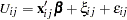
The random utility function of individual for choice can be decomposed into deterministic and stochastic components:

where is a deterministic utility function, assumed to be linear in the explanatory variables, and is an unobserved random variable that captures the factors that affect utility that are not included in . Different assumptions on the distribution of the errors, , give rise to different classes of models.

The features of discrete choice models available in the MDC procedure are summarized in Table 17.1.

IEV stands for type I extreme-value (or Gumbel) distribution with the probability density function and the cumulative distribution function of the random error given by and ; HEV stands for heteroscedastic extreme-value distribution with the probability density function and the cumulative distribution function of the random error given by 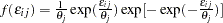and 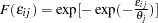, where is a scale parameter for the random component of the th alternative; GEV stands for generalized extreme-value distribution; MVN represents multivariate normal distribution; and is an error component. See the Mixed Logit Model section for more information about .