| The ESM Procedure |
Example 13.1 Forecasting of Time Series Data
This example uses retail sales data to illustrate how the ESM procedure can be used to forecast time series data.
The following DATA step creates a data set from data recorded monthly at numerous points of sales. The data set, SALES, contains a variable DATE that represents time and a variable for each sales item. Each value of the DATE variable is recorded in ascending order, and the values of each of the other variables represent a single time series:
   data sales;
      format date date9.;
      input date : date9. shoes socks laces dresses
                          coats shirts ties belts hats blouses;
   datalines;

   ... more lines ...
The following ESM procedure statements forecast each of the monthly time series:
   proc esm data=sales out=nextyear;
      id date interval=month;
      forecast _numeric_;
   run;
The preceding statements generate forecasts for every numeric variable in the input data set SALES for the next twelve months and store these forecasts in the output data set NEXTYEAR.
The following statements plot the forecasts:
   title1 "Shoe Department Sales";
   proc sgplot data=nextyear;
      series x=date y=shoes / markers
                              markerattrs=(symbol=circlefilled color=red)
                              lineattrs=(color=red);
      series x=date y=socks / markers
                              markerattrs=(symbol=asterisk color=blue)
                              lineattrs=(color=blue);
      series x=date y=laces / markers
                              markerattrs=(symbol=circle color=styg)
                             lineattrs=(color=styg);
      refline '01JAN1999'd / axis=x;
      xaxis values=('01JAN1994'd to '01DEC2000'd by year);
      yaxis values=(2000 to 10000 by 1000) minor label='Websites';
   run;
The plots are shown in Output 13.1.1. The historical data is shown to the left of the reference line and the forecasts for the next twelve monthly periods is shown to the right.
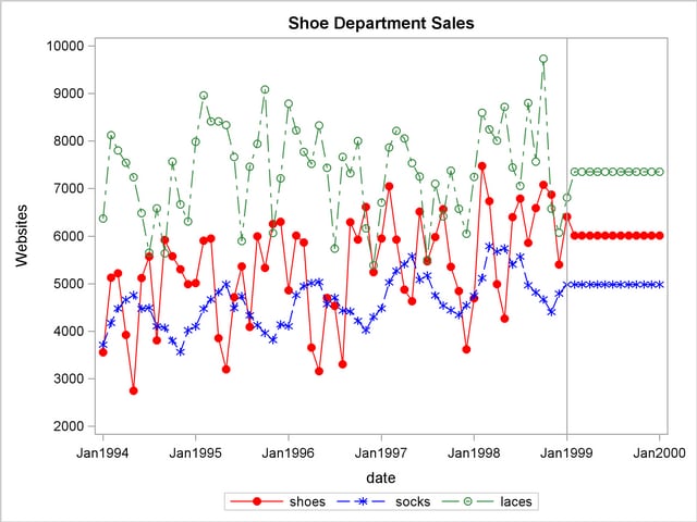
The default simple exponential smoothing model is used because the MODEL= option is omitted on the FORECAST statement. Note that for simple exponential smoothing the forecasts are constant.
The following ESM procedure statements are identical to the preceding statements except that the PRINT=FORECASTS option is specified:
   proc esm data=sales out=nextyear print=forecasts;
      id date interval=month;
      forecast _numeric_;
   run;
In addition to forecasting each of the monthly time series, the preceding statements print the forecasts by using the Output Delivery System (ODS); the forecasts are partially shown in Output 13.1.2. This output shows the predictions, prediction standard errors, and the upper and lower confidence limits for the next twelve monthly periods.
| Forecasts for Variable shoes | |||||
|---|---|---|---|---|---|
| Obs | Time | Forecasts | Standard Error | 95% Confidence Limits | |
| 62 | FEB1999 | 6009.1986 | 1069.4059 | 3913.2016 | 8105.1956 |
| 63 | MAR1999 | 6009.1986 | 1075.7846 | 3900.6996 | 8117.6976 |
| 64 | APR1999 | 6009.1986 | 1082.1257 | 3888.2713 | 8130.1259 |
| 65 | MAY1999 | 6009.1986 | 1088.4298 | 3875.9154 | 8142.4818 |
| 66 | JUN1999 | 6009.1986 | 1094.6976 | 3863.6306 | 8154.7666 |
| 67 | JUL1999 | 6009.1986 | 1100.9298 | 3851.4158 | 8166.9814 |
| 68 | AUG1999 | 6009.1986 | 1107.1269 | 3839.2698 | 8179.1274 |
| 69 | SEP1999 | 6009.1986 | 1113.2895 | 3827.1914 | 8191.2058 |
| 70 | OCT1999 | 6009.1986 | 1119.4181 | 3815.1794 | 8203.2178 |
| 71 | NOV1999 | 6009.1986 | 1125.5134 | 3803.2329 | 8215.1643 |
| 72 | DEC1999 | 6009.1986 | 1131.5758 | 3791.3507 | 8227.0465 |
| 73 | JAN2000 | 6009.1986 | 1137.6060 | 3779.5318 | 8238.8654 |
Copyright © 2008 by SAS Institute Inc., Cary, NC, USA. All rights reserved.