| The AUTOREG Procedure |
| GARCH, IGARCH, EGARCH, and GARCH-M Models |
Consider the series  , which follows the GARCH process. The conditional distribution of the series Y for time t is written
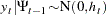 |
where  denotes all available information at time
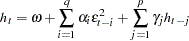
  . The conditional variance
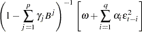
  is
is
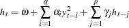 |
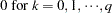
where
 |
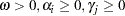 |
The GARCH model reduces to the ARCH
 process when
  . At least one of the ARCH parameters must be nonzero (
 ). The GARCH regression model can be written
 |
 |
 |
where  .
.
In addition, you can consider the model with disturbances following an autoregressive process and with the GARCH errors. The AR -GARCH regression model is denoted
 |
 |
|
|
GARCH Estimation with Nelson-Cao Inequality Constraints
The GARCH model is written in ARCH( ) form as
 |
 |
 |
|||
 |
|
 |
where  is a backshift operator. Therefore,
  if
if  and
and  . Assume that the roots of the following polynomial equation are inside the unit circle:
 |
where  and Z is a complex scalar.
  and
and  do not share common factors. Under these conditions,
  ,
,  , and these coefficients of the ARCH() process are well defined.
Define  . The coefficient
  is written
 |
|
 |
|||
 |
|
 |
|||
 |
|||||
 |
|
 |
|||
 |
|
 |
where  for
for  and
and  for
for  .
.
Nelson and Cao (1992) proposed the finite inequality constraints for GARCH and GARCH
 cases. However, it is not straightforward to derive the finite inequality constraints for the general GARCH model.
For the GARCH model, the nonlinear inequality constraints are
 |
 |
 |
|||
 |
 |
|
|||
|
|
 |
For the GARCH model, the nonlinear inequality constraints are
 |
 |
 |
|||
 |
|
|
|||
 |
 |
|
|||
 |
|
|
|||
|
|
 |
where  and
and  are the roots of
  .
.
For the GARCH model with  , only
 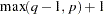 nonlinear inequality constraints (
 for
for  to max(
 )) are imposed, together with the in-sample positivity constraints of the conditional variance
  .
.
Using the HETERO Statement with GARCH Models
The HETERO statement can be combined with the GARCH= option in the MODEL statement to include input variables in the GARCH conditional variance model. For example, the GARCH variance model with two dummy input variables D1 and D2 is
 |
|
 |
|||
 |
|
 |
The following statements estimate this GARCH model:
   proc autoreg data=one;
      model y = x z / garch=(p=1,q=1);
      hetero d1 d2;
   run;
The parameters for the variables D1 and D2 can be constrained using the COEF= option. For example, the constraints  are imposed by the following statements:
   proc autoreg data=one;
      model y = x z / garch=(p=1,q=1);
      hetero d1 d2 / coef=unit;
   run;
Limitations of GARCH and Heteroscedasticity Specifications
When you specify both the GARCH= option and the HETERO statement, the GARCH=(TYPE=EXP) option is not valid. The COVEST= option is not applicable to the EGARCH model.
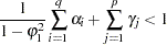
IGARCH and Stationary GARCH Model
The condition 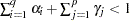 implies that the GARCH process is weakly stationary since the mean, variance, and autocovariance are finite and constant over time. However, this condition is not sufficient for weak stationarity in the presence of autocorrelation. For example, the stationarity condition for an AR(1)-GARCH process is
 |
When the GARCH process is stationary, the unconditional variance of  is computed as
 |
where  and is the GARCH conditional variance.
Sometimes the multistep forecasts of the variance do not approach the unconditional variance when the model is integrated in variance; that is,  .
.
The unconditional variance for the IGARCH model does not exist. However, it is interesting that the IGARCH model can be strongly stationary even though it is not weakly stationary. Refer to Nelson (1990) for details.
EGARCH Model
The EGARCH model was proposed by Nelson (1991). Nelson and Cao (1992) argue that the nonnegativity constraints in the linear GARCH model are too restrictive. The GARCH model imposes the nonnegative constraints on the parameters,  and
and  , while there are no restrictions on these parameters in the EGARCH model. In the EGARCH model, the conditional variance,
  , is an asymmetric function of lagged disturbances
  :
:
 |
where
 |
 |
The coefficient of the second term in  is set to be 1 (
 =1) in our formulation. Note that
  if
if  . The properties of the EGARCH model are summarized as follows:
The function
is linear in  with slope coefficient
  if is positive while is linear in with slope coefficient
  if is negative.
 Suppose that
 . Large innovations increase the conditional variance if
  and decrease.
 the conditional variance if

Suppose that
 . The innovation in variance, , is positive if the innovations are less than
  . Therefore, the negative innovations in returns,
  , cause the innovation to the conditional variance to be positive if
  is much less than 1.
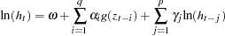
GARCH-in-Mean
The GARCH-M model has the added regressor that is the conditional standard deviation:
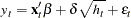 |
|
where follows the ARCH or GARCH process.
Maximum Likelihood Estimation
The family of GARCH models are estimated using the maximum likelihood method. The log-likelihood function is computed from the product of all conditional densities of the prediction errors.
When  is assumed to have a standard normal distribution (
 ), the log-likelihood function is given by
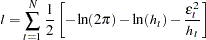 |
where  and is the conditional variance. When the GARCH-M model is estimated,
 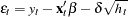 . When there are no regressors, the residuals
  are denoted as or
  .
.
If has the standardized Student’s t distribution, the log-likelihood function for the conditional t distribution is
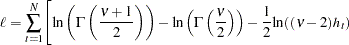 |
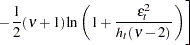 |
where  is the gamma function and
  is the degree of freedom (
 ). Under the conditional t distribution, the additional parameter
  is estimated. The log-likelihood function for the conditional t distribution converges to the log-likelihood function of the conditional normal GARCH model as
  .
.
The likelihood function is maximized via either the dual quasi-Newton or trust region algorithm. The default is the dual quasi-Newton algorithm. The starting values for the regression parameters  are obtained from the OLS estimates. When there are autoregressive parameters in the model, the initial values are obtained from the Yule-Walker estimates. The starting value
  is used for the GARCH process parameters.
The variance-covariance matrix is computed using the Hessian matrix. The dual quasi-Newton method approximates the Hessian matrix while the quasi-Newton method gets an approximation of the inverse of Hessian. The trust region method uses the Hessian matrix obtained using numerical differentiation. When there are active constraints, that is,  , the variance-covariance matrix is given by
 |
where  and
and  . Therefore, the variance-covariance matrix without active constraints reduces to
  .
.
Copyright © 2008 by SAS Institute Inc., Cary, NC, USA. All rights reserved.