Creating a Distribution Analysis

Overview

Use the Distribution Analysis transformation to generate distribution analysis data in a target table and on the Output tab of the Job Editor. The target receives data only for the columns that are involved in the analysis. You can control many aspects of how data is generated, including choosing the type of analysis and which columns are analyzed.

The Distribution Analysis transformation is based on the UNIVARIATE procedure, which is documented in the "The UNIVARIATE Procedure" section in Base SAS Procedures Guide: Statistical Procedures.

The UNIVARIATE procedure provides the following:

descriptive statistics based on moments (including skewness and kurtosis), quantiles or percentiles (such as the median), frequency tables, and extreme values
histograms and comparative histograms. These can also be fitted with probability density curves for various distributions and with threaded kernel density estimates.
quantile-quantile plots (Q-Q plots) and probability plots. These plots facilitate the comparison of a data distribution with various theoretical distributions.
goodness-of-fit tests for a variety of distributions including the normal
the ability to inset summary statistics on plots produced on a graphics device
the ability to analyze data sets with a frequency variable
the ability to create output data sets containing summary statistics, histogram intervals, and parameters of fitted curves

You can use the UNIVARIATE procedure, together with the VAR statement, to compute summary statistics. In addition, you can use the following statements to request plots:

the HISTOGRAM statement for creating histograms, the QQPLOT statement for creating Q-Q plots, and the PROBPLOT statement for creating probability plots.
the CLASS statement together with the HISTOGRAM, QQPLOT, and PROBPLOT statement for creating comparative histograms, Q-Q plots, and probability plots.
the INSET statement with any of the plot statements for enhancing the plot with an inset table of summary statistics. The INSET statement is applicable only to plots produced on graphics devices.

You can specify grouping columns in the Distribution Analysis transformation. Doing so causes a SAS BY statement to order target rows according to the values in the grouping columns. The Distribution Analysis transformation requires that grouping columns be sorted in ascending order in the source. If you specify grouping columns, you can sort those columns before the Distribution Analysis transformation by using a SAS Sort transformation.

Problem

You want to generate a distribution analysis.

Solution

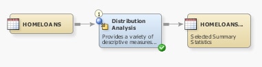
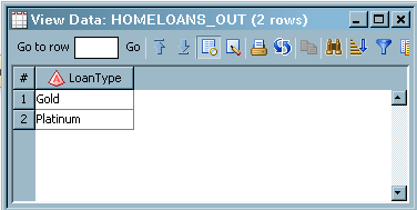
You can use Distribution Analysis transformation as an interface to the UNIVARIATE procedure in a job that generates a distribution analysis and creates an ODS document that contains its results. For example, you can create a job similar to the sample job featured in this topic. This sample job generates a distribution analysis that is based on a table of data about home loans. The output for this job is sent to a target table, the Output tab in the Job Editor window, and an ODS document that is configured in the job. The sample job includes the following tasks:

Create and Populate the Job
Configure Analytical Options
Configure Reporting Options
Run the Job and View the Output

Tasks

Create and Populate the Job

Perform the following steps to create and populate the job:

Create an empty SAS Data Integration Studio job.
Select and drag a Distribution Analysis transformation from the Analysis folder in the Transformations tree. Then, drop it in the empty job on the Diagram tab in the Job Editor window.
Select and drag the source table out of the Inventory tree. Then, drop it before the Distribution Analysis transformation on the Diagram tab.
Drag the cursor from the source table to the input port of the Distribution Analysis transformation. This action connects the source to the transformation.
Right-click the Distribution Analysis transformation, and click Add Output Port from the Ports option in the drop-down menu. This step enables you to add an output port to the transformation.
Select and drag the source table from the Inventory tree. Then, drop it after the Distribution Analysis transformation on the Diagram tab.
Drag the cursor from the Distribution Analysis transformation output port to the target table. This action connects the target to the transformation.

The following display shows a sample process flow diagram for a job that contains the Distribution Analysis transformation.

Sample Process Flow

Note that the source table for the sample job is named HOMELOANS, and the target table is named HomeLoans_out.

Configure Analytical Options

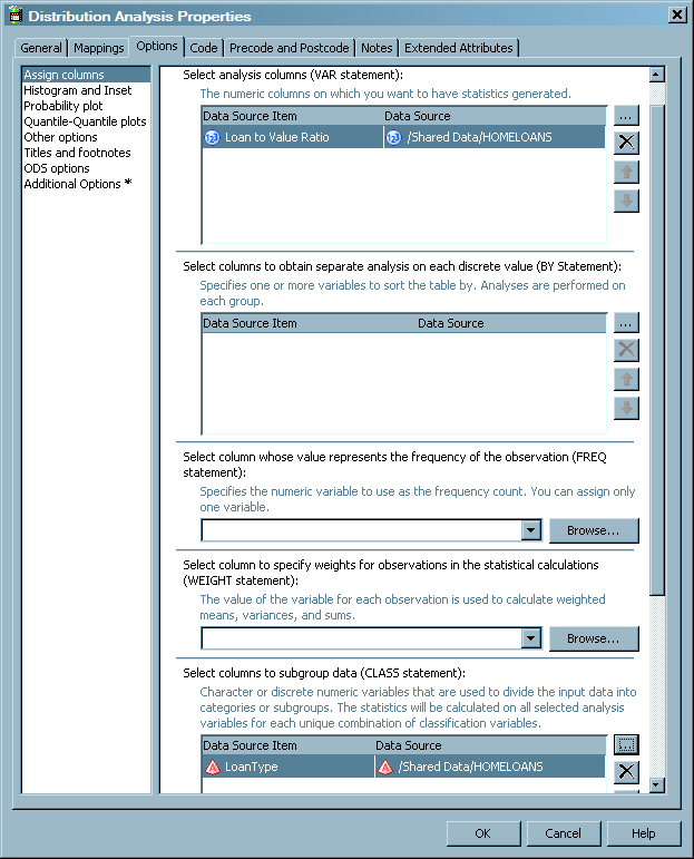
Use the Options tab in the properties window for the Distribution Analysis transformation to configure the output for your analysis. Note that the Options tab is divided into two parts, with a list of categories on the left-hand side and the options for the selected category on the right-hand side. Perform the following steps to set the options that you need for your job:

Open the properties window for the Distribution Analysis transformation on the Diagram tab in the Job Editor window. Then, click the Options tab.
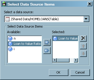
Click Assign columns to access the Assign columns page. Use the column selection prompts to access the columns that you need for your job. For example, you can click for the Select analysis columns (VAR statement) field to access the Select Data Source Items window, as shown in the following display.

Sample Select Data Source Items Window

In the sample job, the VAR statement column is Loan to Value Ratio. The column assignment options are shown in the following display.

Sample Options Properties
Note that you must select the other columns that you need for your job, such as the Loan Type column in the CLASS statement required for the sample job.
Enter the other options that you need for your analysis. In the sample job, options are set in the Histogram and Inset page to generate a histogram for the analysis.

Configure Reporting Options

Use the remaining option pages to create and save a report based on the analysis conducted in the job. Perform the following steps to set the reporting options:

Click Title and footnotes to access the Title and footnotes page and enter up to three headings and two footnotes.
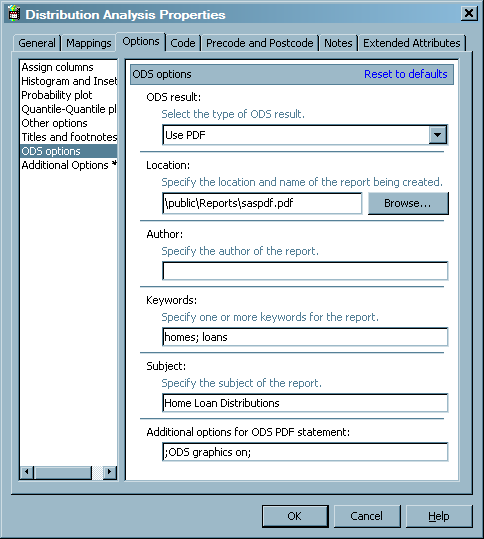
Click ODS options to access the ODS options page. You can choose between HTML, RTF, and PDF output and enter appropriate settings for each. The sample job uses PDF output. Therefore, a location, a set of keywords, the subject of the report, and code to enable ODS graphics are added to the fields that are displayed when Use PDF is selected in the ODS Result field. (The path specified in the Location field is relative to the SAS Application Server that executes the job.) These fields are shown in the following display.

Sample ODS Options
Click OK to save the settings for the Options tabs.

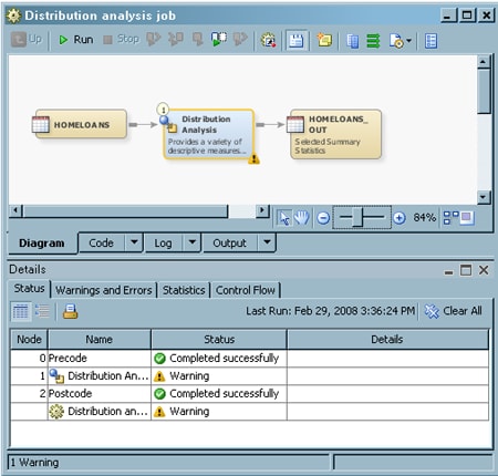
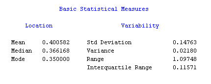
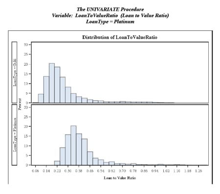
Run the Job and View the Output

Perform the following steps to run the job and view the output:

Right-click on an empty area of the job, and click Run in the pop-up menu. SAS Data Integration Studio generates code for the job and submits it to the SAS Application Server for execution. The following display shows a successful run of a sample job.

Sample Completed Job
If error messages display on the Status tab, read and respond to the messages as needed. The sample jobs display warning messages because ODS graphics are experimental for this transformation. The expected output is still displayed on the Output tab and in the PDF report that is generated in the job.
To view the distribution analysis, click the Output tab in the Job Editor window. If the Output tab is not available, enable it at Tools OptionsShow Output tab in the menu bar. The following display shows a portion of the analysis for the sample job.

Sample Output in the Output Tab
To view the target table, right-click the target and select Open. The following display shows the target table data for the sample job.

Target Table Data
Open the PDF document that you created and saved earlier. The following display shows the histogram generated in a sample report based on the data.

Sample PDF Output