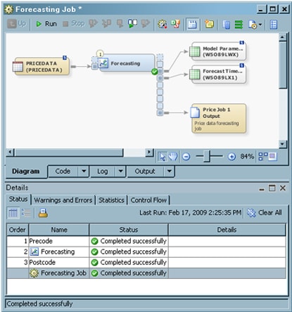
Generating Forecasts

Overview

Use the Forecasting transformation to run the High-Performance Forecasting procedure (PROC HPF) against a warehouse data store. PROC HPF provides a quick and automatic way to generate forecasts for many sets of time series or transactional data. The procedure can forecast millions of series at a time, with the series organized into separate variables or across BY groups. The Forecasting transformation provides a simple interface for entering values for various options that are associated with PROC HPF.

The Forecasting transformation can forecast either time series or transactional data:

Time series data consists or observations that are equally spaced by a specific time interval, such as a month or week.
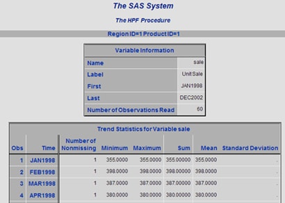
Transactional data consists of observations that are not spaced with respect to any particular time interval. Typical examples of transactional data include information that is drawn from the Internet, inventory, and sales. For transactional data, the data is accumulated based on a specified time interval to form a procedure reference. The transformation can also perform trend and seasonal analysis on this transactional data.

The following prerequisites apply to the Forecasting transformation:

SAS High-Performance Forecasting software must be installed on the SAS Application Server that executes a job that includes the Forecasting transformation.
If you use plot options in the transformation, you will need to have the SAS/GRAPH component installed on the SAS Application Server that executes the job.

Problem

You want to generate a forecast in the context of a SAS Data Integration Studio job.

Solution

You can use the Forecasting transformation. The transformation runs the High-Performance Forecasting procedure (PROC HPF) against a warehouse data store. The options that are included in the Forecasting transformation give you the flexibility to tailor the output to meet your business needs.

PROC HPF provides a quick and automatic way to generate forecasts for many sets of time series or transactional data. Note that SAS High-Performance Forecasting software must be installed on the SAS Application Server that executes a job that includes the Forecasting transformation. Perform the following tasks:

Tasks

Create and Populate the Job

Perform the following steps to create and populate the job:

Create an empty job.
Drop the source table onto the Diagram tab of the Job Editor window.
Select and drag a Forecasting transformation from the Analysis folder in the Transformations tree in the Job Editor window. The following display shows a sample process flow for a forecasting job:

Sample Forecasting Process Flow

Note that the source table is named PRICEDATA. The output document and tables are created during the configuration of the Forecasting transformation.

Set HPF Statement Options

The HPF tab in the properties window of the Forecasting transformation enables you to set options in the HPF statement in PROC HPF. Perform the following steps to set HPF statement options:

Open the HPF tab in the properties window for the Forecasting transformation.
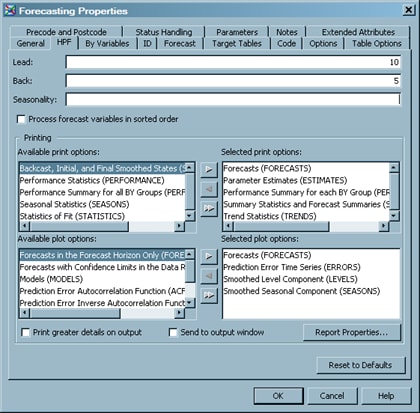
Enter the HPF statement options that you need to generate your forecast. The following display shows the HPF options for a sample job:

Sample HPF Options

Note that the number of the periods preceding and following the forecast are set in the Lead and Back fields for this sample job. Appropriate print and plot options are also set. The print options specify the types of data that are printed in the output. The plot options specify the graphical plots that are included in the output. Use the arrow keys to move between the available options and selected options fields.

Set BY VARIABLE Statement Options

The By Variables tab provides an interface to the BY statement, which you can use to obtain separate analyses for groups of statements defined by the BY variables. Perform the following steps to set BY statement options:

Click By Variable.
Select the appropriate columns from Columns field and move them to the Sort by columns field. For example, the values for the region and products columns are selected in the sample job. Keep the default Ascending sort order setting.

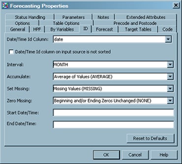
Set ID Statement Options

The ID tab provides an interface to the ID statement, which you can use to designate a numerical variable that identifies observations in the input and output data sets. Perform the following steps to set ID statement options:

Click ID.
Set appropriate values for the ID statement. The following display shows the ID options for a sample job:

Sample ID Options

Note that date is selected in the Data/Time Id Column field for the sample job and that appropriate values are selected in the Interval, Accumulate, Set Missing, and Zero Missing fields. You can also specify start and end dates and times, if appropriate for your forecast.

Set FORECAST Statement Options

The Forecast tab provides an interface to the FORECAST statement, which you can use to list the numeric variables in the data set. The accumulated values in this data set represent the time series that is to be modeled and forecast. Perform the following steps to set FORECAST statement options:

Click Forecast.
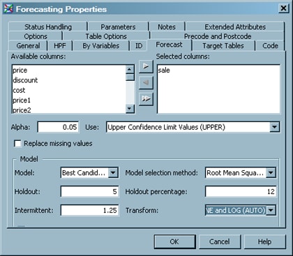
Set appropriate values for the FORECAST statement. The following display shows the forecast options for a sample job:

Sample FORECAST Options

Note that sale is selected in the Selected columns field for the sample forecast. In addition, 0.01 is entered in the Alpha field. This setting specifies the significance level to use in computing the confidence limits of the forecast. The default is ALPHA=0.05, which produces 95% confidence intervals. Similar settings are made in the Use, Model, Model selection method, Intermittent, and Transform fields to support the sample forecast.

Set Target Table Options

The Target Tables tab provides an interface for selecting the tables that are generated in the forecast output. You can select any combination of the tables that are listed on the tab. Perform the following steps to select your target tables:

Click Target Tables.
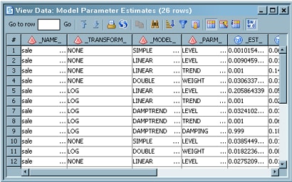
Select the appropriate values for your forecast. Note that the Model Parameter Estimates check box and the Forecast Time Series Components check box are selected in the sample job. Therefore, the Model Parameter Estimates and Forecast Time Series Components target tables are included in the output of the sample forecast.
Click the OK button to save the settings in the Forecasting properties window and return to the Job Editor window.

Configure the Report Output

This configuration ensures that the output is directed to the target tables directory and that the titles of the tables and the HTML document make sense to anyone who needs to review the forecast results. Perform the following steps to configure the output of the forecast HTML document:

Open the properties window for the output document in the forecasting job. Then, click the Details tab.
Enter the path to the directory where you store your target tables in the Path field.
Click OK to save the settings in the properties window and return to the Diagram tab of the Job Editor window.

Run the Job

Perform the following steps to run the forecasting job:

Right-click on an empty area of the job, and click Run in the pop-up menu. SAS Data Integration Studio generates code for the job and submits it to the SAS Application Server for execution.
If error messages display, read and respond to the messages as needed. The following display shows a completed forecasting job:

Sample Completed Forecasting Job

View the Output

Perform the following steps to verify that the job created the desired output:

Right-click the output document in the Diagram tab, and click Open in the pop-up menu. The output file in the sample job is named Price Job 1 Output. (You might be prompted to enter a user ID and password for the server that accesses the table.)
The HTML output of the forecast is displayed in your default Web browser. This file contains two types of output: tabular data and graphical plots. The following display shows the sample tabular data:

Sample Forecast Table

The following display shows a sample graphical plot:

Sample Forecast Plot
Right-click the first target table on the Diagram tab, and click Open in the pop-up menu. The following display shows the data for the target table in the View Data window:

Sample Target Table Data

Note: The target tables in the sample job are temporary output tables that are not preserved when the SAS session is ended. If you need permanent target tables, right-click the target tables and click Replace in the pop-up menu.
Repeat the process for the other target tables in your forecast.