Differences among Predictive Modeling Nodes

The Regression node, the Tree node, and the Neural Network node can all learn complex models from data, but they have different ways of representing complexity in their models. Choosing a model of appropriate complexity is important for making accurate predictions, as discussed in the section below on Generalization. Simple models are best for learning simple functions of the data (as long as the model is correct, of course), while complex models are required for learning complex functions. With all data mining models, one way to increase the complexity of a model is to add input variables. Other ways to increase complexity depend on the type of model:

One fundamental difference between tree-based models and both regression and neural net models is that tree-based models learn step functions, whereas the other models learn continuous functions. If you expect the function to be discontinuous, a tree-based model is a good way to start. However, given enough data and training time, neural networks can approximate discontinuities arbitrarily well. Polynomial regression models are not good at learning discontinuities. To model discontinuities using regression, you need to know where the discontinuities occur and construct dummy variables to indicate the discontinuities before fitting the regression model.

For both regression and neural networks, the simplest models are linear functions of the inputs. Hence regression and neural nets are both good for learning linear functions. Tree-based models require many branches to approximate linear functions accurately.

When there are many inputs, learning is inherently difficult because of the curse of dimensionality (see the Neural Network FAQ at ftp://ftp.sas.com/pub/neural/FAQ2.html#A_curse.

To learn general nonlinear functions, all modeling methods require a degree of complexity that grows exponentially with the number of inputs. That is, as the number of inputs increases, the number of interactions and polynomial terms required in a regression model grows exponentially, the number of hidden units required in a neural network grows exponentially, and the number of branches required in a tree grows exponentially. The amount of data and the amount of training time required to learn such models also grow exponentially.

Fortunately, in most practical applications with a large number of inputs, most of the inputs are irrelevant or redundant, and the curse of dimensionality can be circumvented. Tree-based models are especially good at ignoring irrelevant inputs, since trees often use a relatively small number of inputs even when the total number of inputs is large.

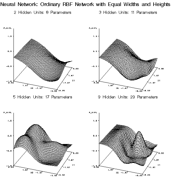
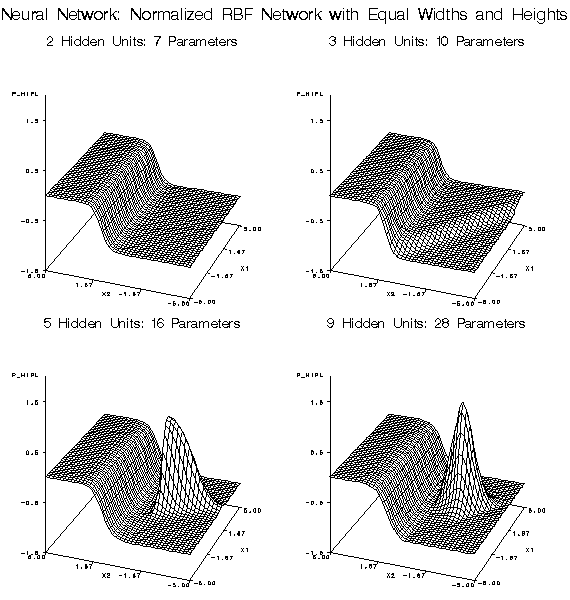
If the function to be learned is linear, stepwise regression is good for choosing a small number out of a large set of inputs. For nonlinear models with many inputs, regression is not a good choice unless you have prior knowledge of which interactions and polynomial terms to include in the model. Among various neural net architectures, multilayer perceptrons and normalized radial basis function (RBF) networks are good at ignoring irrelevant inputs and finding relevant subspaces of the input space, but ordinary radial basis function networks should be used only when all or most of the inputs are relevant.

All of the modeling nodes can process redundant inputs effectively. Adding redundant inputs has little effect on the effective dimensionality of the data. Hence the curse of dimensionality does not apply. When there are redundant inputs, the training cases lie close to some (possibly nonlinear) subspace. If this subspace is linear, redundancy is called multicollinearity.

In statistical theory, it is well-known that redundancy causes parameter estimates (weights) to be unstable. That is, different parameter estimates can produce similar predictions. But if the purpose of the analysis is prediction, unstable parameter estimates are not necessarily a problem. If the same redundancy applies to the test cases as to the training cases, the model needs to produce accurate outputs only near the subspace occupied by the data, and stable parameter estimates are not needed for accurate prediction. However, if the test cases do not follow the same pattern of redundancy as the training cases, generalization will require extrapolation and will rarely work well.

If extrapolation is required, decision tree-based models are safest, because trees choose just one of several redundant inputs and produce constant predictions outside the range of the training data. Stepwise linear regression or linear-logistic regression are the next safest methods for extrapolation if a large singularity criterion is used to make sure that the parameter estimates do not become excessively unstable. Polynomial regression is usually a bad choice for extrapolation, because the predictions will often increase or decrease rapidly outside the range of the training data. Neural networks are also dangerous for extrapolation if the weights are large. Weight decay and early stopping can be used to discourage large weights. Normalized radial basis function (RBF) networks are the safest type of neural net architecture for extrapolation, since the range of predictions will never exceed the range of the hidden-to-output weights.

The Decision Tree node can use cases with missing inputs for training and provides several ways of making predictions from cases with missing inputs. The Regression and Neural Network nodes cannot use cases with missing inputs for training; predictions are based on the unconditional mean or prior probabilities. (See Predicted Values and Posterior Probabilities.)

The Neural Network node can model two or more target variables in the same network. Having multiple targets in the network can be an advantage when there are features common to all the targets. Otherwise, it is more efficient to train separate networks. The Regression node and the Decision Tree node process only one target at a time, but the Start Group node can be used to handle multiple targets.

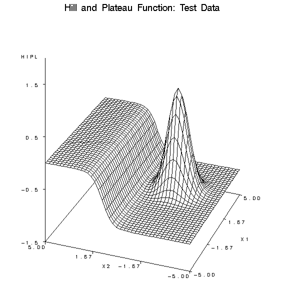
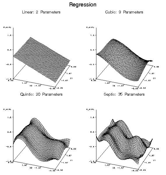
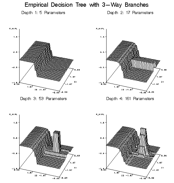
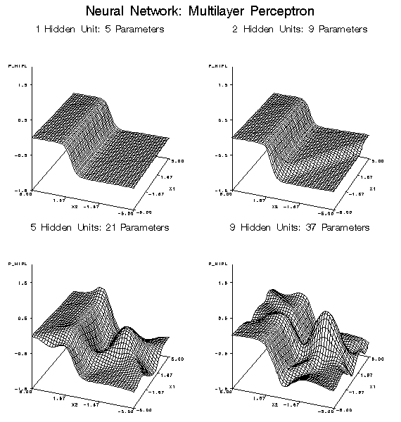
The following figures illustrate the types of approximation error that commonly occur with each of the modeling nodes. The noise-free data come from the hill-and-plateau function, which was chosen because it is difficult for typical neural networks to learn. Given sufficient model complexity, all of the modeling nodes can, of course, learn the data accurately. These examples show what happens with insufficient model complexity. The cases in the training set lie on a 21 by 21 grid, while those in the test set are on a 41 by 41 grid.