Decision Thresholds and Profit Charts
-
Using a profit chart to set a decision threshold. For this approach, there is an implicit decision (usually a decision to "do nothing") that is not included in the decision matrix. The decisions made in the modeling nodes are tentative. The profit and loss summary statistics from the modeling nodes are not used. Instead, you look at profit charts (similar to lift or gains charts) in the Model Comparison node to decide on a threshold for the do-nothing decision. Then you use a Transform Variables or SAS Code node that sets the decision variable to "do nothing" when the expected profit or loss is not better than the threshold chosen from the profit chart. This approach is popular for business applications such as direct marketing.
To understand the difference
between these two approaches to decision making, you first need to
understand the effects of various types of transformations of decisions
on the resulting decisions and summary statistics.
Consider the formula
for the expected profit of decision d in case i using (without loss
of generality) revenue and cost:
![A(i,d) = Sum(i)Q(i,t,d)Post(i,t) = Sum(i)[Revenue(t,d) – Cost(i,d)]Post(i,t) = Sum(i)Revenue(t,d)Post(i,t) – Cost(i,d)Sum(t)Post(i,t)](images/prede117.png)
Now transform the decision
problem by adding a constant to the tth row of the revenue matrix and a constant ci to the ith row of the cost matrix, yielding
a new expected profit A'(i,d):
![A’(i,d) = Sum(t)[Revenue(t,d) + r(sub-t)]Post(i,t) – [Cost(i,d) + c(sub-i)]Sum(t)Post(i,t) = A(i,d) + Sum(i)r(sub-i)Post(i,t) + c(sub-i)](images/prede118.png)
In the last expression
above, the second and third terms do not depend on the decision. Hence,
this transformation of the decision problem will not affect the choice
of decision.
![Total Profit = Sum(i)F(i)C(i) = Sum(i)F(i)Q(i,T(i), D(i)) = Sum(i)F(i)[Revenue(T(i), D(i)) – Cost(i, D(i))]](images/prede119.png)
![Total Profit’ = Sum(i)F(i)[Revenue(T(i), D(i)) + r(sub-i) – Cost(i,D(i)) – c(sub-i)] = Sum(i)F(i)[r(sub-i) – c(sub-i)]](images/prede120.png)
In the last expression
above, the second term does not depend on the posterior probabilities
and therefore does not depend on the model. Hence, this transformation
of the decision problem adds the same constant to the total profit
regardless of the model, and the transformation does not affect the
choice of models based on total profit. The same conclusion applies
to average profit and to total and average loss, and also applies
when the adjustment for prior probabilities is used.
For example, in the
German credit benchmark data set (SAMPSIO.DMAGECR), the target variable
indicates whether the credit risk of each loan applicant is good or
bad, and a decision must be made to accept or reject each application.
It is customary to use the loss matrix:
This loss matrix says
that accepting a bad credit risk is five times worse than rejecting
a good credit risk. But this matrix also says that you cannot make
any money no matter what you do, so the results might be difficult
to interpret (or perhaps you should just get out of business). In
fact, if you accept a good credit risk, you will make money, that
is, you will have a negative loss. And if you reject an application
(good or bad), there will be no profit or loss aside from the cost
of processing the application, which will be ignored. Hence, it would
be more realistic to subtract one from the first row of the matrix
to give a more realistic loss matrix:
This loss matrix will
yield the same decisions and the same model selections as the first
matrix, but the summary statistics for the second matrix will be easier
to interpret.
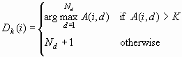
Sometimes a decision
threshold K is used to modify the decision-making process, so that
no decision is made unless the maximum expected profit exceeds K.
However, making no decision is really a decision to make no decision
or to "do nothing." Thus. the use of a threshold implicitly creates
a new decision numbered Nd+1. Let Dk(i) be the decision based on threshold K. Thus:
If the decision and
cost matrices are correctly specified, then using a threshold is suboptimal,
since D(i) is the optimal decision, not Dk(i).
But a threshold-based decision can be reformulated as an optimal decision
using modified decision and cost matrices in several ways.
A threshold-based decision
is optimal if "doing nothing" actually yields an additional revenue
K. For example, K might be the interest earned on money saved by doing
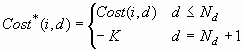
nothing. Using the profit matrix formulation, you can define an augmented
profit matrix Profit* with Nd+1 columns, where:
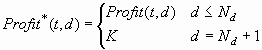
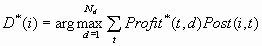
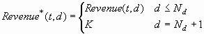
Then D*(i) = DK(i). Equivalently, you can define augmented revenue
and cost matrices, Revenue*> and Cost*, each with Nd+1 columns, where:

A threshold-based decision
is also optimal if doing anything other than nothing actually incurs
an additional cost K. In this situation, you can define an augmented
profit matrix Profit* with Nd+1 columns, where:
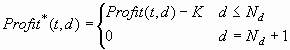
This version of Profit*
produces the same decisions as the previous version, but the total
profit is reduced by  regardless of the model used. Similarly, you can
define Revenue* and Cost* as:
regardless of the model used. Similarly, you can
define Revenue* and Cost* as:
regardless of the model used. Similarly, you can
define Revenue* and Cost* as:
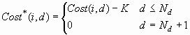
Again, this version
of the Revenue* and Cost* matrices produces the same decisions as
the previous version, but the total profit is reduced by regardless of the model used.
regardless of the model used.
If you want to apply
a known decision threshold in any of the modeling nodes in Enterprise
Miner, use an augmented decision matrix as described above. If you
want to explore the consequences of using different threshold values
to make suboptimal decisions, you can use profit charts in the Model
Comparison node with a non-augmented decision matrix. In a profit
chart, the horizontal axis shows percentile points of the expected
profit E(i). By the default, the deciles of E(i) are used to define
10 bins with equal frequencies of cases. The vertical axis can display
either cumulative or noncumulative profit computed from C(i).
To see the effect on
total profit of varying the decision threshold K, use a cumulative
profit chart. Each percentile point p on the horizontal axis corresponds
to a threshold K equal to the corresponding percentile of E(i). That
is:
![p/100 =[( Sum(i|E(i)<K) F(i))/(Sum(i) F(i))]](images/prede130.png)
However, the chart shows
only p, not K. Since the chart shows cumulative profit, each case
with E(i) < K contributes a profit of C(i), while all other cases
contribute a profit of zero. Hence, the ordinate (vertical coordinate)
of the curve is the total profit for the decision rule Dk(i), assuming that the profit for the decision to do
nothing is zero:

Transformations that
add a constant  to the tth row of the
revenue matrix or a constant ci to the ith row of the cost matrix can change the expected profit
for different cases by different amounts and therefore can alter the
order of the cases along the horizontal axis of a profit chart, producing
large changes in the cumulative profit curve.
to the tth row of the
revenue matrix or a constant ci to the ith row of the cost matrix can change the expected profit
for different cases by different amounts and therefore can alter the
order of the cases along the horizontal axis of a profit chart, producing
large changes in the cumulative profit curve.