Analyze with a Logistic Regression Model

As part of your analysis, you want to include some parametric models for comparison with the decision trees that you built in Build Decision Trees. Because it is familiar to the management of your organization, you have decided to include a logistic regression as one of the parametric models.

To use the Regression node to fit a logistic regression model:

Select the Model tab on the Toolbar.
Select the Regression node icon. Drag the node into the Diagram Workspace.
Connect the Transform Variables node to the Regression node.
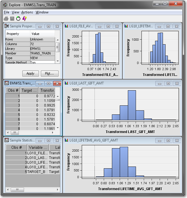
To examine histograms of the imputed and transformed input variables, right-click the Regression node and select Update. In the diagram workspace, select the Regression node. In the Properties Panel, scroll down to view the Train properties, and click on the ellipses that represent the value of Variables. The Variables — Reg window appears.
1. Select all variables that have the prefix LG10_. Click Explore. The Explore window appears.
  
  You can select a bar in any histogram, and the observations that are in that bucket are highlighted in the EMWS.Trans_TRAIN data set window and in the other histograms. Close the Explore window to return to the Variables — Reg window.
2. (Optional) You can explore the histograms of other input variables.
3. Close the Variables — Reg window.
In the Properties Panel, scroll down to view the Train properties. Click on the Selection Model property in the Model Selection subgroup, and select Stepwise from the drop-down menu that appears. This specification causes SAS Enterprise Miner to use stepwise variable selection to build the logistic regression model.

Note: The Regression node automatically performs logistic regression if the target variable is a class variable that takes one of two values. If the target variable is a continuous variable, then the Regression node performs linear regression.
In the Diagram Workspace, right-click the Regression node, and select Run from the resulting menu. Click Yes in the Confirmation window that opens.
In the window that appears when processing completes, click Results. The Results window appears.
Maximize the Output window. This window details the variable selection process. Lines 401 – 424 list a summary of the steps that were taken.
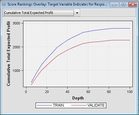
Minimize the Output window and maximize the Score Rankings Overlay window. From the drop-down menu, select Cumulative Total Expected Profit.

The data that is used to construct this plot is ordered by expected profit. For this example, you have defined a profit matrix. Therefore, expected profit is a function of both the probability of donation for an individual and the profit associated with the corresponding outcome. A value is computed for each decision from the sum of the decision matrix values multiplied by the classification probabilities and minus any defined cost. The decision with the greatest value is selected, and the value of that selected decision for each observation is used to compute overall profit measures.

The plot represents the cumulative total expected profit that results from soliciting the best n% of the individuals (as determined by expected profit) on your mailing list. For example, if you were to solicit the best 40% of the individuals, the total expected profit from the validation data would be approximately $1850. If you were to solicit everyone on the list, then based on the validation data, you could expect approximately $2250 profit on the campaign.
Close the Results window.