Perform Reject Inference on the Model

The preliminary scorecard that was built in the previous section used known good and bad loans from only the accepted applicants. The scorecard modeler needs to apply the scorecard to all applicants, both accepted and rejected. The scorecard needs to generalize the “through the door” population. In this section, you perform reject inference to solve the sample bias problem so that the developmental sample will be similar to the population to which the scorecard will be applied.

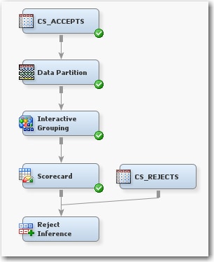
From the Credit Scoring tab, drag a Reject Inference node into the Diagram Workspace. Connect the Scorecard node to the Reject Inference node.
From the Project Panel, drag the CS_REJECTS data source into the Diagram Workspace. Connect the CS_REJECTS data set to the Reject Inference node.
The Reject Inference node attempts to infer the behavior (good or bad), or performance, of the rejected applicants using three industry-accepted inference methods. You can set the inference method using the Inference Method property.
The following inference methods are supported in SAS Enterprise Miner:
- Fuzzy — Fuzzy classification uses partial classifications of “good” and “bad” to classify the rejected applicants in the augmented data set. Instead of classifying observations as “good” and “bad,” fuzzy classification allocates weight to observations in the augmented data set. The weight reflects the observation's tendency to be “good” or “bad.”
  
  The partial classification information is based on the probability of being good or bad based on the model built with the CS_ACCEPTS data set that is applied to the CS_REJECTS data set. Fuzzy classification multiplies these probabilities by the user-specified Reject Rate parameter to form frequency variables. This results in two observations for each observation in the Rejects data. Let p(good) be the probability that an observation represents a good applicant and p(bad) be the probability that an observation represents a bad applicant. The first observation has a frequency variable defined as (Reject Rate)*p(good) and a target variable of 0. The second observation has a frequency variable defined as (Reject Rate)*p(bad) and a target value of 1.
  
  Fuzzy is the default inference method.
- Hard Cutoff — Hard Cutoff classification classifies observations as either good or bad based on a cutoff score. If you choose Hard Cutoff as your inference method, you must specify a Cutoff Score in the Hard Cutoff properties. Any score below the hard cutoff value is allocated a status of bad. You must also specify the Rejection Rate in General properties. The Rejection Rate is applied to the CS_REJECTS data set as a frequency variable.
- Parceling — Parceling distributes binned, scored rejected applicants into either a good bin or a bad bin. Distribution is based on the expected bad rates that are calculated from the scores from the logistic regression model. The parameters that must be defined for parceling vary according to the Score Range method that you select in the Parceling properties group. All parceling classifications require that you specify the Rejection Rate, Score Range Method, Min Score, Max Score, and Score Buckets properties.
You must specify a value for the Rejection Rate property when you use either the Hard Cutoff or Parceling inference method. The Rejection Rate is used as a frequency variable. The rate of bad applicants is defined as the number of bad applicants divided by the total number of applicants. The value for the Rejection Rate property must be a real number between 0.0001 and 1. The default value is 0.3.

The Cutoff Score property is used when you specify Hard Cutoff as the inference method. The Cutoff Score is the threshold score that is used to classify good and bad observations in the Hard Cutoff method. Scores below the threshold value are assigned a status of bad; all other observations are classified as good.
The Parceling properties group is available when you specify Parceling as the inference method.
The following properties are available in the Parceling properties group:
- Score Range Method — Use the Score Range Method property to specify how you want to define the range of scores to be bucketed. The available methods are as follows:
  
  Accepts — The Accepts score range method distributes the rejected applicants into equal-sized buckets based on the score range of the CS_ACCEPTS data set.
  
  Rejects — The Rejects score range method distributes the rejected applicants into equal-sized buckets based on the score range of the CS_REJECTS data set.
  
  Scorecard — The Scorecard score range method distributes the rejected applicants into equal-sized buckets based on the score range that is output by the augmented data set.
  
  Manual — The Manual score range method distributes the rejected applicants into equal-sized buckets based on the range that you input.
- Score Buckets — Use the Score Buckets property to specify the number of buckets that you want to use to parcel the data set into during attribute classification. Permissible Score Buckets property values are integers between 1 and 100. The default setting for the Score Buckets property is 25.
When you use the Parceling inference method, you must also specify the Event Rate Increase property. The proportion of bad and good observations in the CS_REJECTS data set is not expected to approximate the proportion of bad and good observations in the CS_ACCEPTS data set. Logically, the bad rate of the CS_REJECTS data set should be higher than that of the CS_ACCEPTS data set. It is appropriate to use some coefficient to classify a higher proportion of rejected applicants as bad. When you use Parceling, the observed event rate of the accepts data is multiplied by the value of the Event Rate Increase property to determine the event rate for the rejects data. To configure a 20% increase, set the Event Rate Increase property to 1.2.
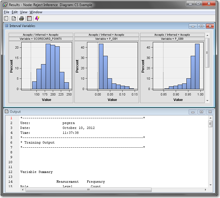
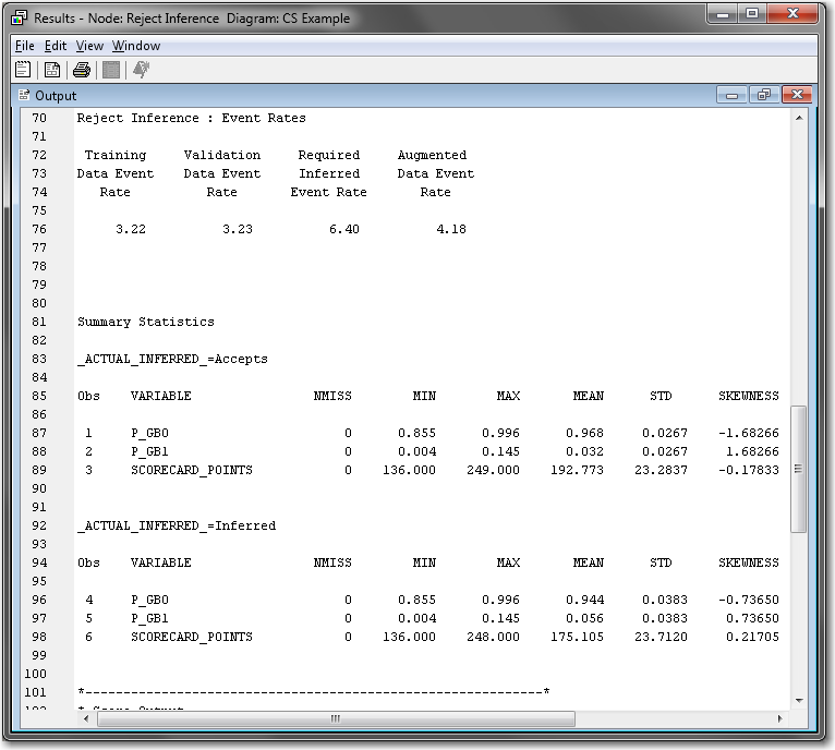
For this example, you will use the default values for the Reject Inference node properties. Right-click the Reject Inference node and select Run. In the Confirmation window, select Yes.
In the Run Status window, select Results.

The Results window includes distribution plots for the score and predicted probabilities for the accepted observations and the inferred samples side-by-side.

Expand the Output window. Scroll down to the Reject Inference: Event Rates section to the event rates for various samples, including the augmented data.

The output from the Reject Inference node is the augmented data, with both CS_ACCEPTS and CS_REJECTS appended together. The Training Data Event Rate and the Validation Data Event Rate are the event rates (that is, the bad rates) for the accepted applicant’s data set. The Required Inferred Event Rate is the event rate for the rejected applicant’s data set. The Augmented Data Event Rate is the event rate for the augmented data set. The Summary Statistics sections display basic summary statistics for both the accepted and rejected applicants’ data.

When you are done analyzing the Reject Inference node output, close the Results window.