Group the Characteristic Variables into Attributes

You will now use the Interactive Grouping node to perform variable grouping, which is a binning transformation performed on the input variables. Variable grouping is also referred to as classing.

From the Credit Scoring tab, drag an Interactive Grouping node onto the Diagram Workspace. Connect the Data Partition node to the Interactive Grouping node.

The Interactive Grouping node performs the initial grouping automatically. You can use these initial groupings as a starting point to modify the classes interactively. By default, the unbinned interval variables are grouped into 20 quantiles (also called bins), which are then grouped based on a decision tree. The Interactive Grouping node enables you to specify the properties of this decision tree.
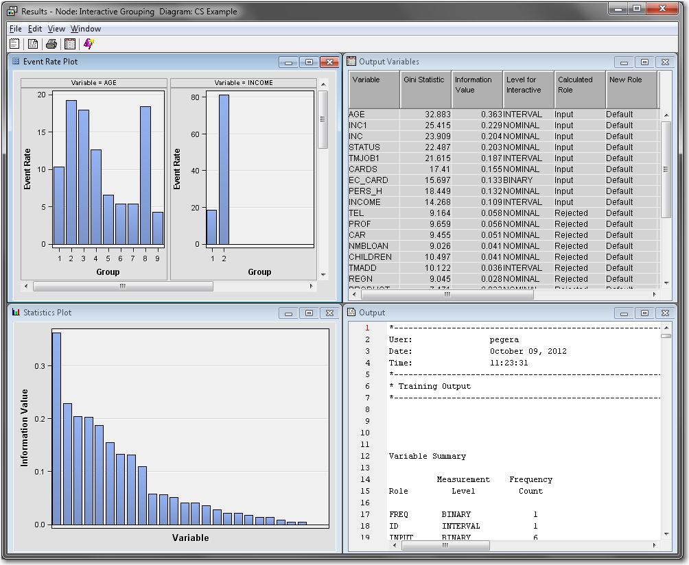
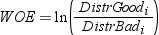
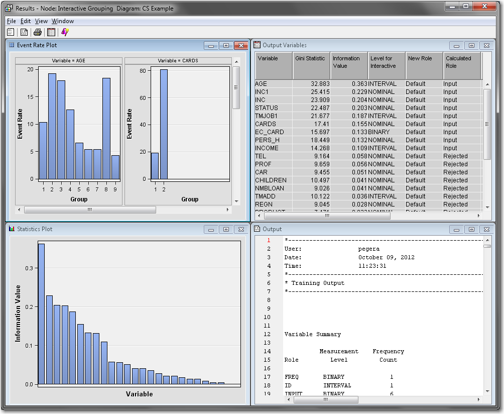
Select the Interactive Grouping node in the Diagram Workspace. Set the value of the Interval Grouping Method property and the Ordinal Grouping Method property to Monotonic Event Rate.

Set the value of the Maximum Number of Groups property to 10.
Right-click the Interactive Grouping node and select Run. In the Confirmation window that appears, click Yes. In the Run Status window that appears, click Results.

The Output Variables window displays each variable’s Gini Statistic and information value (IV). Note that a variable receives an Exported Role of Rejected if the variable’s IV is less than 0.10. Recall that IV is used to evaluate a characteristic’s overall predictive power (that is, the characteristic’s ability to separate between good and bad loans). Information value is calculated as follows:

Here L is the number of attributes for the characteristic variable. In general an IV less than 0.02 is unpredictive, a value between 0.02 and 0.10 is weakly predictive, a value between 0.10 and 0.30 is moderately predictive, and a value greater than 0.30 is strongly predictive.

The Gini statistic is used as an alternative to the IV. The formula for the Gini statistic is more complicated than the IV and can be found in the SAS Enterprise Miner help documentation.

In the Properties Panel of the Interactive Grouping node, you can specify the cutoff values for the Gini and IV statistics. For example, the default IV cutoff of 0.10 for rejecting a characteristic can be changed to another value using the Information Cutoff Value property.

The Statistics Plot window shows a bar chart of each variable against its information value. You can move your cursor over a bar to display tooltip information, which includes the variable name, IV, and variable role.

Based on the IV, the variables AGE, INC1, INC, STATUS, TMJOB1, CARDS, EC_CARD, PERS_H, and INCOME are considered the candidate inputs to build the final scorecard in the regression step. The IV and Gini statistics might change if the groupings of the attributes are changed. The initial, automatic binning provides a good starting point to create the groupings for the scorecard, but the groupings can be fine-tuned.

Close the Results window.
Now that you have run the node, you can open the Interactive Grouping application. Click the button in the Interactive Grouping property. This opens the Interactive Grouping window.

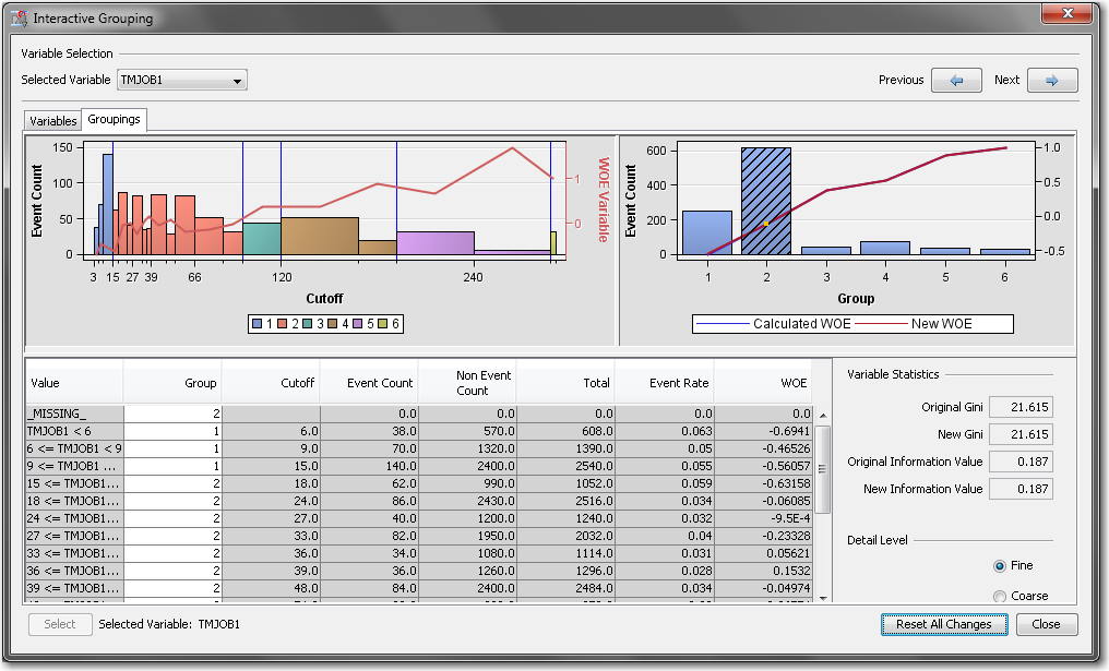
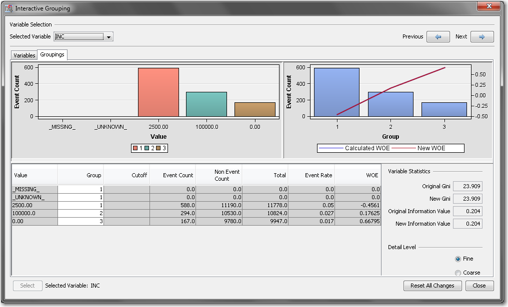
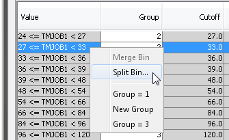
By default, the variables are sorted by their information value, given in the Original Information Value column. Also, the variable that is selected by default is the variable with the greatest IV. In this example, that variable is AGE.

Use the drop-down menu in the upper left corner of the Interactive Grouping window to select the variable TMJOB1. The variable TMJOB1 represents the applicant’s time at their current job.

Select the Groupings tab in the Interactive Grouping window.

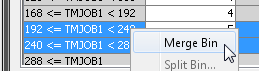
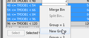
The plot on the right shows the weights of evidence for each group of the variable INC. Recall that the weight of evidence (WOE) measures the strength of an attribute of a characteristic in differentiating good and bad accounts. Weight of evidence is based on the proportion of good applicants to bad applicants at each group level. For each group i of a characteristic WOE is calculated as follows:

Negative values indicate that a particular grouping is isolating a higher proportion of bad applicants than good applicants. That is, negative WOE values are worse in the sense that applicants in that group present a greater credit risk. By default, missing values are assigned to their own group. The shape of the WOE curve is representative of how the points in the scorecard are assigned. As you can see on the Groupings tab, as time on the job increases, so does WOE.

The plot on the left shows the details of each group for the selected variable. It shows the distribution of the bad loans within each group.

You can use the table to manually specify cutoff values. Suppose that you want to make 30 a cutoff value in the scorecard. Select the row that contains 30 in the score range, as shown below.

In the Split Bin window, enter 30 in the Enter New Cutoff Value dialog box. Click OK. Note that Group 2 now contains another bin that has a cutoff value of 30.

You can also use the Groupings tab to combine multiple bins within a group. Suppose that you want to combine the two bins in Group 5 into a single bin. Select the rows that correspond to Group 5, right-click one of the rows, and select Merge Bin.

Note that Group 5 now contains just one bin.

Finally, you can use the Groupings tab to create a new group from the defined bins. Suppose that you want Group 2 to contain fewer observations. Select the last four rows of Group 2, where the value of TMJOB1 is between 48 and 96, and then right-click the node and select New Group.

Note that there are now 7 groups, but this change did not have a significant impact on the WOE curve.

In general, changes to your grouping or binning will affect the WOE graph. For example, there might be a characteristic input that should have increasing, monotonic WOE values for each group. If the auto-binning of the Interactive Grouping node does not find these groupings, then the ability to fine-tune the groupings to achieve a monotonic WOE graph can be quite powerful.

The Interactive Grouping node can create groups that are based on several binning techniques, including statistically optimal ones. The user has the ability to change these bins based on business knowledge and known bias in the data to make the WOE trends logical. The changes previously made are suggested only if the analyst has expert knowledge and has a specific reason for changing the bins of a characteristic variable.

Also, after changes are made in the Interactive Grouping node as shown above, it is possible that the statistics for WOE, IV, and Gini can change. Some of the variables that were examined in the Results window might now not be candidates for input into the scorecard based on the IV and Gini statistics.

Close the Interactive Grouping window. Select Yes in the Save Changes window.
In the Diagram Workspace, right-click the Interactive Grouping node and select Results. Compare the new results to those observed earlier.

Notice that the original candidate variables are still candidate variables after the changes that you made in the Interactive Grouping window. Close the Results window.