Understanding the Load-Balancing Algorithms
Overview
The following algorithms
support load balancing on SAS workspace server, stored process servers,
pooled workspace servers, and OLAP servers:
-
(SAS Workspace Servers and SAS Stored Process Servers only) The cost algorithm assigns a cost value (determined by the administrator) to each client that connects to the server. The algorithm can also assign cost values to servers that have not started yet. When a new client requests a connection, load balancing redirects the client to the connection with the lowest cost on the machine with the lowest total cost. This is the default algorithm for stored process and standard workspace servers.
-
(SAS Stored Process Servers only) Each spawner's load balancer maintains an ordered list of machines and their response times. Load balancing updates this list periodically at an interval that is specified by the administrator. When a new client requests a connection, load balancing redirects the client request to the machine at the top of the list.
-
The Grid algorithm communicates with a SAS Grid Manager to allow load balancing access to grid-related load information. This information is used by the object spawner to find the least loaded server machine that will accept the client request. (This algorithm is available only when the SAS Grid Server has been deployed.)
-
(SAS Pooled Workspace Servers only) The Most Recently Used algorithm emphasizes reusing workspace servers. This algorithm attempts to send clients into running servers before starting new servers. The goal of this algorithm is to reduce the overhead of starting new servers by using servers that are already running. This is the default algorithm for pooled workspace servers.
Cost Algorithm: Overview
The Cost algorithm uses a cost value to represent the
work load that is assigned to each server (or server process) in the
load-balancing cluster. Each time a client connects or a stored process
is executed, the spawner updates the cost value for the appropriate
server. When a client requests a connection to the load-balancing
cluster, the spawner examines the cost values for all of the servers
in the cluster, and then redirects the client to the server that has
the lowest cost value.
The Cost algorithm supports
SAS Workspace Servers and SAS Stored Process Servers only. This algorithm
works differently depending on the server type:
-
SAS Workspace Servers. The cost algorithm uses the server with the lowest cost on the host with the lowest cost.When a new client requests a connection, the load-balancing spawner redirects the client to the server that has the lowest cost value. When the client connects to the designated server, the spawner increments that server's cost by a specified value (cost per client). When that client disconnects, the spawner decrements that server's cost by the same value (cost per client).
-
SAS Stored Process Servers. The cost algorithm uses the server process with the lowest cost on the host with the lowest cost.When a new client requests a connection, the load-balancing spawner redirects the client to the server process that has the lowest cost value on the machine with the lowest total cost. When the client connects to the designated server process, the spawner increments the cost for that process by the same value (cost per client).The stored process server cost is determined by three values: the cost per client is used when the client connects; session cost; and server context cost. The default values for session and context costs are 1 and 100 respectively. To change the default values, use the Options tab in the properties window of the logical stored process server.
Cost Algorithm: Parameters
Cost per client
(field on the load-balancing
logical server definition) specifies the default amount of weight
(cost) that each client adds (when it connects) or subtracts (when
it disconnects) to the total cost of the server.
Startup cost
(field on the server
definition) specifies the start-up cost of the server. When a request
is made to the load-balancing spawner, the spawner assigns this start-up
cost value to inactive servers. A new server is not started unless
it is determined that its cost (the start-up cost) is less than that
of the rest of the servers in the cluster. This field enables the
administrator to control the order in which servers are started. After
a server is started, the cost value is 0. When a client connects to
the server, the server's cost value is increased.
Cost Algorithm: SAS Workspace Server Example
A load balancing cluster
contains two workspace servers on two different machines, Machine
A and Machine B. The following table displays the initial status of
the cluster:
At the start of the
example, five clients have connected to the cluster and the client
connections are balanced between the two servers. Workspace Server
A has three clients and Workspace Server B has two clients. The following
figure illustrates what happens when an additional client requests
a connection:
New Client Connection
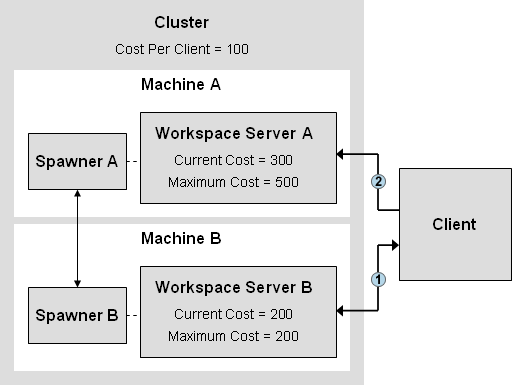
| 1 | The client requests a connection to Workspace Server B. The spawner on Machine B examines the cost values of all of the servers in the cluster. Workspace Server B has the least cost, but it has reached its Maximum Cost value and cannot accept any more clients. The spawner redirects the client to Workspace Server A. |
| 2 | The client requests a connection to Workspace Server A. The spawner on Machine A creates a server connection for the client, and then increments the cost value for Workspace Server A by the cluster's Cost Per Client value (100). |
Cost Algorithm: SAS Stored Process Server Example
A load-balancing cluster
contains one stored process server with two server processes (MultiBridge
connections), Server Process A and Server Process B. The following
table displays the initial status of the cluster:
At the start of the
example, Server Process A is running and has two clients. Each client
on Server Process A is running one stored process, so the cost to
connect for Server A is 402 (2 clients * 100 + 2 stored processes
running * 101). 100 represents the cost per client. 101 represents
the context cost (100) and the session cost (1).
Server Process B has
not started yet, so the cost to connect to Server Process B is the
Startup Cost (300). The following figure illustrates what happens
when an additional client connects:
New Client Connection
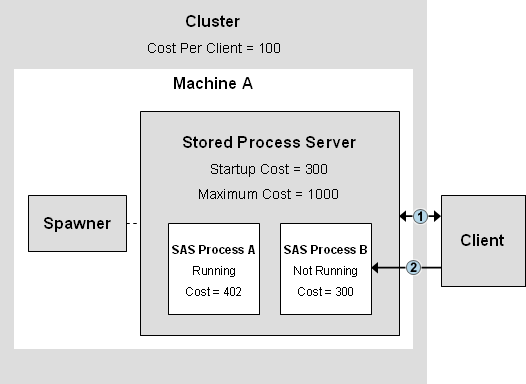
| 1 | The client requests a connection to the stored process server. The load-balancing spawner examines the cost values of all of the servers in the cluster and determines that Server Process B has the lowest cost. The spawner redirects the client to Server Process B. |
| 2 | The client requests a connection to Server Process B. The spawner starts the server process and then provides a connection to the client. The spawner increments the cost value for Server Process B by the cluster's Cost Per Client value (100). |
At the end of the example,
the cost for Server Process B is 100, because there is one client
and the Cost Per Client value is 100. There are no stored processes
running, and the Startup Cost value does not apply because the server
process has been started. If the client submits a stored process,
the cost will increase by 101 (the standard cost per stored process).
Response Time Algorithm
The Response Time algorithm uses a list
of server response times in order to determine which server process
has the least load. For each server process in the load-balancing
cluster, the load-balancing spawner maintains an ordered list of servers
and their average response times. Each time the spawner receives a
client request, it redirects the client to the server process at the
top of the list. The spawner updates the server response times periodically.
You can specify the update frequency for the response time (response
refresh time) in the metadata for the load-balancing cluster.
Refresh rate
(field on the load-balancing
logical server definition) specifies the length of the period in milliseconds
that the load-balancing spawner will use the current response times.
At the end of this period the spawner updates the response times for
all of the servers in the cluster and then reorders the list of servers.
Grid Algorithm
If you have a SAS grid installed and configured, then
you can leverage the functionality of the SAS Grid Manager to identify
the SAS IOM server best suited to handle a SAS client's request in
your cluster of workspace servers. The Grid algorithm communicates
with a SAS Grid Manager to allow load-balancing access to grid-related
load information. This information is used by the object spawner or
the OLAP server to find the least loaded server machine that will
accept the client request.
Grid server
(field on the load-balancing
logical server definition) specifies the name of the SAS Grid Server
with which the object spawner gathers grid-related load information.
Most Recently Used (MRU) Algorithm
The Most Recently Used algorithm
emphasizes reusing workspace servers. This algorithm attempts to send
clients into running servers before starting new servers. The goal
of this algorithm is to reduce the overhead of starting new servers
by using servers that are already running.
Least Recently Used (LRU) Algorithm
The Least Recently Used (LRU)
algorithm attempts to use the least recently used server. This algorithm
balances provides more of a breadth-first approach to balancing the
client load.
MRU and LRU Algorithms: Pooled Workspace Server Examples
Overview of MRU and LRU Algorithm Examples
The topics in this section
examine three examples of load balancing a pooled workspace server
using the Most Recently Used (MRU) and Least Recently Used (LRU) load-balancing
algorithms:
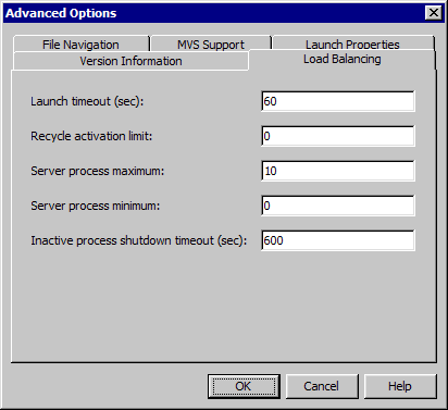
Example 1: Default LRU and MRU Settings
This pool manages a
maximum of 10 clients concurrently. Each server process accepts only
one client at a time. The Server Process Maximum property
determines how many processes can be started. If a client disconnects
from one of the servers in the pool, the process continues running
and is returned to the pool. The reuse of the server from the pool
is determined by the load-balancing algorithm.
The LRU algorithm attempts
to use the least recently used server. LRU pools tend to grow faster
because the processes that are not running are at the top of the list
when looking at least recently used processes.
The MRU algorithm attempts
to use a server that was recently used. MRU pools try to reuse processes
rather than start new ones, but they will start new processes as needed,
up to the maximum. Server processes in the pool that are inactive
shut down after 10 minutes (600 seconds). There is no minimum set
on this pool, so all the processes in this pool can time out if they
are inactive.