| Overview |
Your Results
When you click OK in the Simple Linear Regression dialog, the output from a simple linear regression is automatically displayed in the Analysis window. Drag the borders of the Analysis window until you can see all of the output.
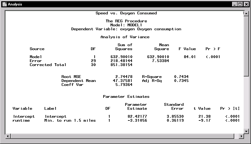 |
Figure 1.6: Simple Regression Output
This model might be considered minimally adequate with an R-square value of 0.7434; the negative coefficient for runtime indicates that the linear relationship between oxygen consumption and running time is a negative one.
You can save and print your results from this window. You can also copy your output to the Program Editor window, where you can copy it to the clipboard and paste it into other applications.
Close the Analysis window to see the project tree. In addition to output, a scatter plot and the SAS code used to perform the regression and create the scatter plot are displayed as nodes in the project tree by default.
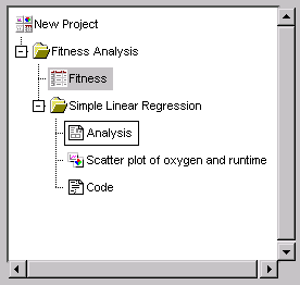 |
Figure 1.7: Results in Project Tree
Double-click on the Scatter plot node to view the scatter plot that you have created.
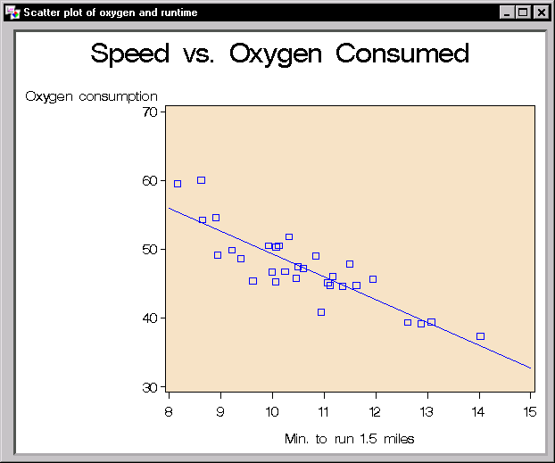 |
Figure 1.8: Scatter Plot
The scatter plot illustrates the results of your simple linear regression: higher oxygen consumption rates are associated with lower running times. You can change the graph to fit the window, edit the graph, or save it to a different format, such as GIF, by selecting File ![]() Save As ...
Save As ...
Close the Scatter Plot window to view the Code node in the project tree.
Double-click on the Code node to view the SAS code that was used to perform the simple linear regression and create the scatter plot.
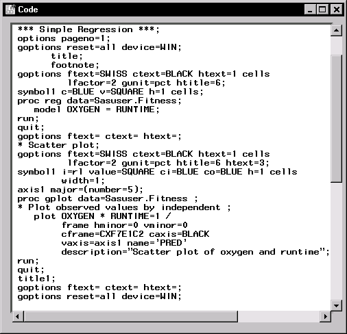 |
Figure 1.9: Code
Copyright © 2007 by SAS Institute Inc., Cary, NC, USA. All rights reserved.