Repeated Measures

Repeated Measures Analysis

The data set analyzed in this task contains data from Littell, Freund, and Spector (1991). Subjects in the study participated in one of three different weightlifting programs, and their strength was measured once every other day for two weeks after they began the program. The first program increased the number of repetitions as the subject became stronger (RI), the second program increased the amount of weight as subjects became stronger (WI), and the subjects in the third program did not participate in weightlifting (CONT). The objective of this analysis is to investigate the effect each weightlifting program has on increasing strength over time. This section also illustrates how to prepare data in univariate form for this task.

Open the Weightsmult Data Set

The data are provided in the Analyst Sample Library. To open the Weightsmult data set, follow these steps:

Select Tools Sample Data ...
Select Weightsmult.
Click OK to create the sample data set in your Sasuser directory.
Select File Open By SAS Name ...
Select Sasuser from the list of Libraries.
Select Weightsmult from the list of members.
Click OK to bring the Weightsmult data set into the data table.

Data Management

Figure 16.2 displays the Weightsmult data in multivariate form, which means that a single row in the data table contains all response measurements for a single subject. The Program variable defines the treatment group and takes the values `CONT', `RI', and `WI'. The Subject variable defines each subject, and the variables s1 through s7 contain strength measurements across time for each subject.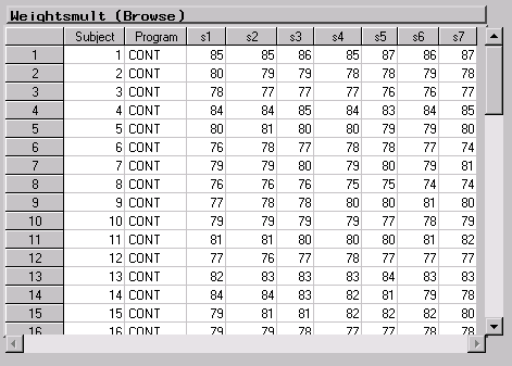

Figure 16.2: Weightsmult Data

In order for you to perform the repeated measures analysis using the Analyst Application, your data must be in univariate form, which means that each response measurement is contained in a separate row. If your data are not in univariate form, you must create a new data table with this structure. This can be accomplished via the Stack Columns task in the Data menu.

The Stack Columns task creates a new table by stacking specified columns into a single column. The values in the other columns are preserved in the new table, and a source column in the new data set contains the names of the columns in the original data set that contained the stacked values.

You want to put the values for columns corresponding to the strength measurement variables s1 through s7 in individual rows, so you want to stack columns s1-s7. To stack the columns, follow these steps:

Select Data Stack Columns ...
Select s1 through s7 and click on the Stack button.
Type Strength in the Stacked column: field.
Click OK to produce the new data set.

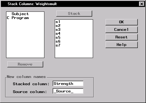Figure 16.3: Stack Columns Dialog

The new data set is presented in the project tree under the Stack Columns folder. The Weightsmult with Stacked Columns folder contains the new data set with the Strength stacked column, and the Code node contains the SAS programming statements that generated the data set.

If a view of the Weightsmult with Stacked Columns data is displayed, close it. Then right-click on the data set node labeled Weightsmult with Stacked Columns, as displayed in Figure 16.4, and select Open to bring the new data set into the data table.

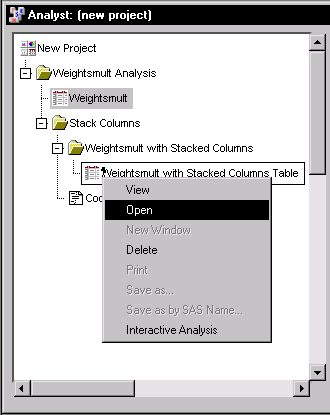Figure 16.4: Stack Columns: Project Tree

The stacked columns data set contains two new variables. The Strength variable contains the strength measurements, and the _Source_ variable denotes the measurement times with seven distinct character values: s1, s2, s3, s4, s5, s6, and s7. However, in this analysis, time needs to be numeric. You can create a numeric variable called Time by using the Recode Values facility.

To create the Time variable, follow these steps:

Select Edit Mode Edit.
Select Data Transform Recode Values ...
Select _Source_ as the Column to recode.
Type Time in the New column name: field.
Specify the new column type by selecting Numeric.
Click OK to enter values of the Time variable that correspond to current values of the _Source_ variable.

Figure 16.5: Recode Values Information Dialog

Type 1 in the New Value (Numeric) column cell next to s1.
Type in the remaining numeric values corresponding to the original values of the _Source_ column. Figure 16.6 displays the final recoded values.
Click OK to create the new variable.

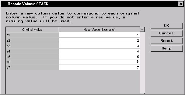Figure 16.6: Recode Values Dialog

The data set now includes a variable Time that contains numeric values for the time of strength measurement. Because the time values are contained in a new variable, you can delete the original variable from the data set by right-clicking on the _Source_ column in the data table and selecting Delete. Once you have deleted the column, the data set should contain four variables, Subject, Program, Strength, and Time, as displayed in Figure 16.7.

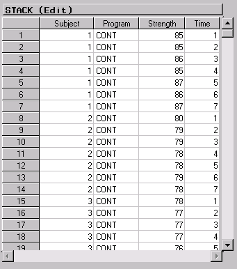Figure 16.7: Weightsuni Data

Before proceeding with the analysis, you can save the new data set as Weightsuni by following these steps:

Select any cell in the data table or reselect the data set node labeled Weightsmult with Stacked Columns in the project tree.
Select File Save As By SAS Name ...
Type Weightsuni in the Member Name field and click Save to save the data set.

Note that the Weightsuni data are in univariate form and should be the same as the Weights data available in the Analyst Sample Library.

Request the Repeated Measures Analysis

To specify the Repeated Measures task, follow these steps:

Select Statistics ANOVA Repeated Measures ...
Select Strength as the dependent variable.
Select Subject, Program, and Time as classification variables.

Figure 16.8 displays the dialog with Strength specified as the dependent variable and Subject, Program, and Time specified as classification variables.

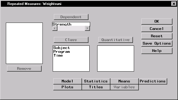Figure 16.8: Repeated Measures Dialog

Define the Model

To perform a repeated measures analysis, you are required to specify a model, define subjects, specify a repeated effect, and select one or more structures for modeling the covariance of the repeated measurements. By defining a factorial structure between Program and Time, you can analyze the between-subject effect Program, the within-subject effect Time, and the interaction between Program and Time.

Each experimental unit, a subject, needs to be uniquely identified in the Weightsuni data set. The value of the Subject variable for the first subject in each separate Program is 1, the value of the Subject variable for the second subject in each Program is 2, and so on. Because subjects participating in different programs have the same value from the Subject variable, you need to nest Subject within Program to uniquely define each subject.

To define the repeated measures model, follow these steps:

Click on the Model button.
Select the Subjects tab.
Select Subject and click Add.
Select Program and click Nest to nest subjects within weightlifting programs.

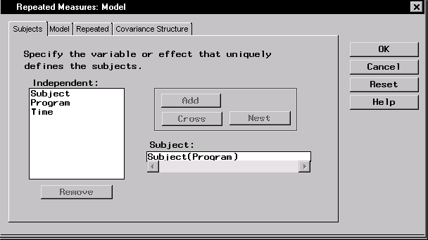Figure 16.9: Repeated Measures: Model Dialog,Subjects Tab

Select the Model tab.
Select Program and Time and click Factorial to specify a factorial arrangement, which is the main effects for Program and Time and their interaction.

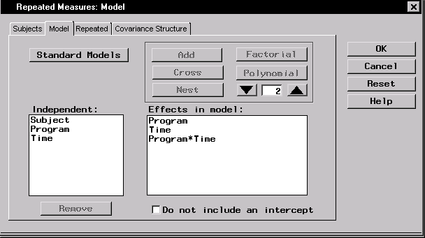Figure 16.10: Repeated Measures: Model Dialog,Model Tab

Select the Repeated tab.
Select Time and click Add to specify measurement times as the repeated effect.

This identifies the repeated measurement effect.

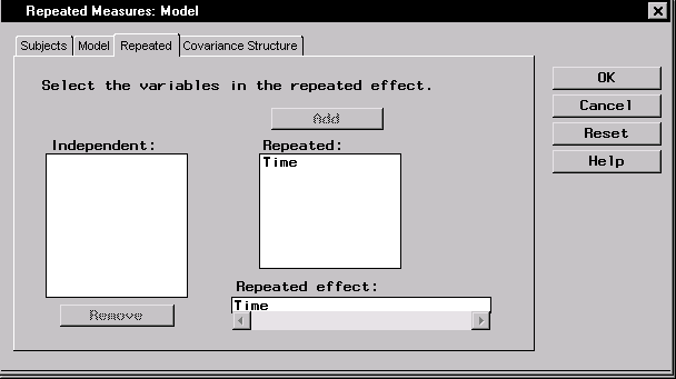Figure 16.11: Repeated Measures: Model Dialog,Repeated Tab

When analyzing repeated measures data, you must properly model the covariance structure within subjects to ensure that inferences about the mean are valid. Using the Repeated Measures task, you can select from a wide range of covariance types, where the most common types are compound symmetric, first-order autoregressive, and unstructured. To select the covariance structure for the analysis, follow these steps:

Select the Covariance Structure tab.
Select the Compound symmetry covariance structure.

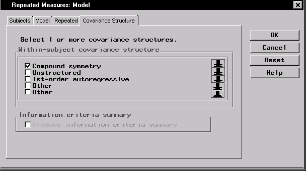Figure 16.12: Repeated Measures: Model Dialog,Covariance Structure Tab

Close the Model dialog by clicking OK. When you have completed your selections, click OK in the main dialog to produce your analysis.

Review the Results

The results are presented in the project tree under the Repeated Measures ANOVA folder, as displayed in Figure 16.13. The nodes represent the repeated measures results and the SAS programming statements (labeled Code) that generated the output.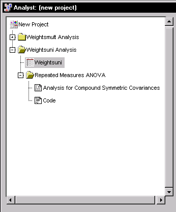

Figure 16.13: Repeated Measures: Project Tree

You can double-click on the Analysis for Compound Symmetric Covariances node in the project tree to view the results in a separate window.

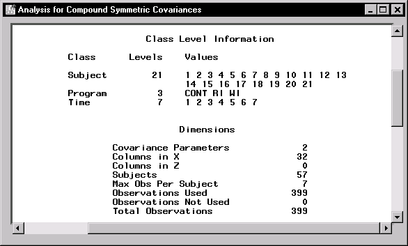Figure 16.14: Repeated Measures: Model Information

Figure 16.14 displays model information including the levels of each classification variable in the analysis. The Program variable has three levels while the Time variable has 7 levels. The "Dimensions" table displays information about the model and matrices used in the calculations. There are two covariance parameters estimated using the compound symmetry model: the variance of residual error and the covariance between two observations on the same subject. The 32 columns of the X matrix correspond to three columns for the Program variable, seven columns for the Time variable, 21 columns for the Program*Time interaction, and a single column for the intercept. You should always review this information to ensure that the model has been specified correctly.

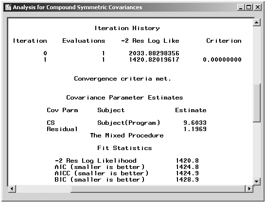Figure 16.15: Repeated Measures: Fitting Information

Figure 16.15 displays fitting information, including the iteration history, covariance parameter estimates, and likelihood statistics. The "Iteration History" table shows the sequence of evaluations to obtain the restricted maximum likelihood estimates of the variance components.

The "Covariance Parameter Estimates" table displays estimates of the variance component parameters. The covariance between two measurements on the same subject is 9.6. Based on an estimated residual variance parameter of 1.2, the overall variance of a measurement is estimated to be 9.6 + 1.2 = 10.8.

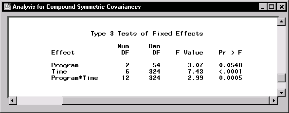Figure 16.16: Repeated Measures: Tests for Fixed Effects

The "Type 3 Tests of Fixed Effects" table in Figure 16.16 contains hypothesis tests for the significance of each of the fixed effects, that is, those effects you specify on the Model tab. Based on a p-value of 0.0005 for the Program*Time interaction, there is significant evidence of a strong interaction between the weightlifting program and time of measurement at the $\alpha = 0.05$ level of significance.

Exploring Alternative Covariance Structures

Based on the assumption of the compound symmetry covariance structure, any two measurements on the same subject have the same covariance regardless of the length of the time interval between the measurements. However, repeated measurements are often more correlated when the measurements are closer in time than when they are farther apart. In this case, compound symmetry may not be appropriate, and you may want to investigate alternative covariance structures.

The first-order autoregressive covariance structure has the property that observations on the same subject that are closer in time are more highly correlated than measurements at times that are farther apart. The first-order autoregressive covariance can be represented by $\sigma^2 \rho^w$ , where w indicates the time between two measurements, $\rho$ stands for the correlation between adjacent observations on the same subject, and $\sigma^2$ stands for the variance of an observation. For the first-order autoregressive covariance structure, the correlation between two measurements decreases exponentially as the length of time between the measurements increases.

To fit an additional repeated measures model with a first-order autoregressive covariance structure, follow these steps:

Select Statistics ANOVA Repeated Measures ...

Note that the selections for the previous analysis are still specified.

Click on the Model button.
Select the Covariance Structure tab.
Select the 1st-order autoregressive structure.
Select Provide information criteria summary to produce a summary table of model-fit criteria for the two covariance structures.
Click OK in the main dialog to produce your analysis.

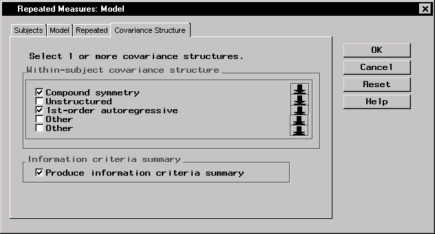Figure 16.17: Repeated Measures: Model Dialog,Covariance Structure tab

Although this analysis models only two different covariance structures, the Analyst Application provides a wide range of structures to choose from, including unstructured, Huynh-Feldt, Toeplitz, and variance components. To select other structures, click on the down arrow next to an Other check box and choose from the resulting drop-down list.

Double-click on the Analysis for First Order Autoregressive Covariances node in the project tree to view the results in a separate window.

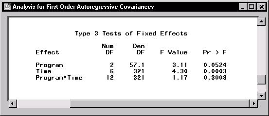Figure 16.18: Repeated Measures: Test for Fixed Effects for Autoregressive Covariance

Figure 16.18 displays the Type 3 tests for fixed effects based on the first-order autoregressive covariance model. Note that with a p-value greater than 0.30, the Program*Time interaction is not significant at the $\alpha = 0.05$ level of significance. The p-value is different from the p-value of the same test based on the compound symmetry covariance structure, and the two models lead to different conclusions. You can assess the model fit based on different covariance structures by comparing criteria that is provided in the Information Criteria Summary window in Figure 16.19.

Figure 16.19: Repeated Measures: Information Criteria Summary

The process of selecting the most appropriate covariance structure can be aided by comparing the Akaike's Information Criterion (AIC) and Schwarz's Bayesian Criterion (SBC) for each model. When you compare models with the same fixed effects but different variance structures, the models with the smallest AIC and SBC are deemed the best. In this example, the autoregressive model has lower values for both AIC and SBC, showing considerable improvement over the model with a compound symmetry structure. Based on the information criteria as well as the intuitively sensible property of the correlations being larger for nearby times than for far-apart times, the first-order autoregressive model is the more suitable fit for these data.

Top of Page