Mixed Models

Clustered Data

The example in this section contains information on a study investigating the heights of individuals sampled from different families. The response variable Height measures the height (in inches) of 18 individuals that are classified according to Family and Gender. Since the data occurs in clusters (families), it is very likely that observations from the same family are statistically correlated and not independent. In this case, it is inappropriate to analyze the data using a standard linear model.

A simple way to model the correlation is through the use of a Family random effect. The Family effect is assumed to be normally distributed with mean of zero and some unknown variance. Defining Family as a random effect sets up a common correlation among all observations having the same level of family.

In addition, a female within a certain family may exhibit more correlation with other females in that same family than with the males in that family, and likewise for males. Defining Family*Gender as a random effect models an additional correlation for all observations having the same value of both Family and Gender.

Open the Heights Data Set

These data are provided as the Heights data set in the Analyst Sample Library. To open the Heights data set, follow these steps:

Select Tools Sample Data ...
Select Heights.
Click OK to create the sample data set in your Sasuser directory.
Select File Open By SAS Name ...
Select Sasuser from the list of Libraries.
Select Heights from the list of members.
Click OK to bring the Heights data set into the data table.

Specify the Mixed Models Analysis

To request a mixed models analysis, follow these steps:

Select Statistics ANOVA Mixed Models ...
Select Height as the dependent variable.
Select Family and Gender as classification variables.
Click Model to open the Model dialog.
Ensure that the Fixed effects check box is selected.
Select Gender and click Add.
Select the Random effects check box, and then select Family and click Add.
Select Family and Gender, and click Cross.
Click OK to return to the main dialog.

Based on your selections, the Mixed Models task constructs the X matrix by creating indicator variables for the Gender effect and including a column of 1s to model the global intercept. The Z matrix contains indicator variables for both the Family effect and the Family*Gender interaction.

Produce a Residual Plot

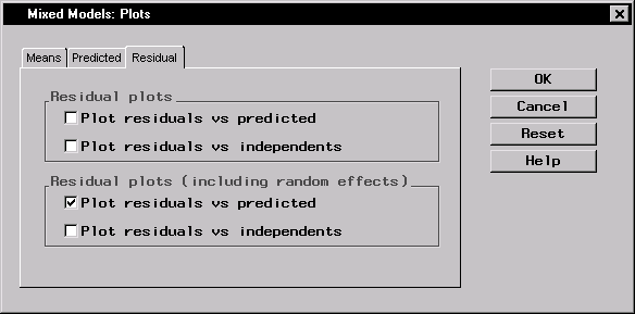
The Mixed Models task can produce means plots for fixed main effects and interactions, plots of predicted values, and residual plots that include or do not include random effects. To produce a plot of residuals versus predicted values that includes random effects, follow these steps:

Click Plots to open the Plots dialog.
Click on the Residual tab, and select Plot residuals vs predicted in the Residual plots (including random effects) box.

Figure 15.9: Mixed Model: Plots Dialog

When you have completed your selections, click OK in the main dialog to perform the analysis.

Review the Results

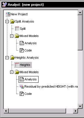
The results are presented in the project tree under the Heights data in the Mixed Models folder, as displayed in Figure 15.10. The three nodes represent the mixed models results, the plot of residuals versus predicted values, and the SAS programming statements (labeled Code) that generate the output.

Figure 15.10: Mixed Models: Project Tree

Double-click on the Analysis node in the project tree to view the contents in a separate window.

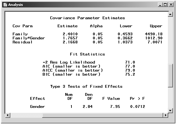
Figure 15.11: Mixed Models: Analysis Results

Figure 15.11 displays the mixed models analysis results for the clustered Heights data. The covariance parameter estimates for Family, Family*Gender, and the residual variance are 2.4, 1.8, and 2.2, respectively. The "Test of Fixed Effects" table contains a significance test for the single fixed effect, Gender. With a p-value of 0.0712, the Type 3 test of Gender is not significant at the $\alpha=0.05$ level of significance. Note that the denominator degrees of freedom for the Type 3 test are computed using a general Satterthwaite approximation. A benefit of performing a random effects analysis using both Family and Family*Gender as random effects is that you can make inferences about gender that apply to an entire population of families, not necessarily to the specific families in this study.

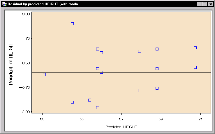
Figure 15.12: Mixed Models: Residuals Plot

Figure 15.12 displays a plot of the residuals versus predicted values that includes random effects, $y-X \hat{\beta} - Z \hat{\gamma}$ versus $X \hat{\beta} + Z \hat{\gamma}$ . Plots are useful for checking model assumptions and identifying potential outlying and influential observations. Based on the plot in Figure 15.12, the data seem to exhibit relatively constant variance across predicted values, and there do not appear to be any outliers or influential observations.

Top of Page