Mixed Models

Split Plot Experiment

One of the most common mixed models is the split-plot design. The split-plot design involves two experimental factors, A and B. Levels of A are randomly assigned to whole plots (main plots), and levels of B are randomly assigned to split plots (subplots) within each whole plot. The subplots are assumed to be nested within the whole plots so that a whole plot consists of a cluster of subplots and a level of A is applied to the entire cluster. The design provides more precise information about B than about A, and it often arises when A can be applied only to large experimental units.

The hypothetical data set analyzed in this example was created as a balanced split-plot design with the whole plots arranged in a randomized complete-block design (Stroup 1989). The response variable Y represents crop growth measurements. The variable A is a whole plot factor that represents irrigation levels for large plots, and the subplot variable B represents different crop varieties planted in each large plot. The levels of B are randomly assigned to split plots (subplots) within each whole plot. The data set Split contains the whole plot factor A, split plot factor B, response Y, and blocking factor Block. Using the Mixed Models task, you can estimate variance components for Block, A*Block, and the residual and automatically incorporate correct error terms into the tests for fixed effects.

Open the Split Data Set

These data are provided as the Split data set in the Analyst Sample Library. To open the Split data set, follow these steps:

Select Tools Sample Data ...
Select Split.
Click OK to create the sample data set in your Sasuser directory.
Select File Open By SAS Name ...
Select Sasuser from the list of Libraries.
Select Split from the list of members.
Click OK to bring the Split data set into the data table.

Request the Mixed Models Analysis

To specify the split plot analysis, follow these steps:

Select Statistics ANOVA Mixed Models ...
Select Y as the dependent variable.
Select A, B, and Block as classification variables.

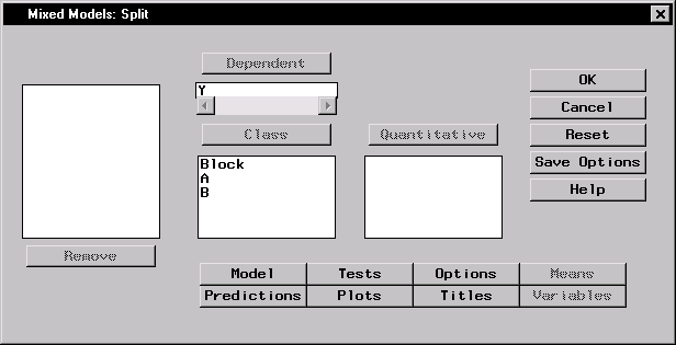Figure 15.2: Mixed Models Dialog

Figure 15.2 displays the dialog with Y specified as the dependent variable and A, B, and Block specified as classification effects in the mixed model.

Specify the Mixed Model

You can define fixed and random effects, create nested terms, and specify interactions in the Model dialog. The Analyst Application adds terms to the Fixed effects list or the Random effects list depending on whether the check box at the top of each list is checked. Check the appropriate box for each term you add. Only classification variables can be specified as random effects, and once a term has been specified as a random effect, all higher-order interactions that include that effect must also be specified as random effects.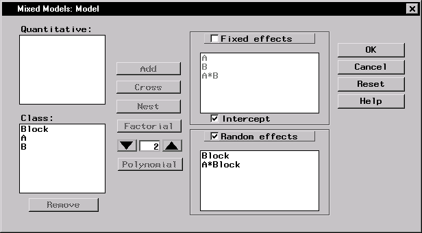

Figure 15.3: Mixed Models: Model Dialog

To specify the mixed model, follow these steps:

Click Model in the main dialog.
Ensure that the Fixed effects check box is selected.
Select A and B and click Factorial.
Select the Random effects check box, and then select Block and click Add.
Select Block and A and click Cross.

These selections create a factorial structure that contains the A and B main effects and the A*B interaction as fixed effects, and Block and A*Block as random effects. Since you specified the random effects, the columns of the model matrix Z now consist of indicator variables corresponding to the levels of Block and A*Block. The G matrix is diagonal and contains the variance components of Block and A*Block; the R matrix is also diagonal and contains residual variance.

Produce Least-Squares Means

You can request generalized least-squares means of fixed effects using the Means dialog. The least-squares means are estimators of the class or subclass marginal means that are expected for a balanced design. Each least-squares mean is computed as ${L\hat{\beta}}$ , where L is the coefficient matrix associated with the least-squares mean and ${\hat{\beta}}$ is the estimate of the fixed-effects parameter vector. Least-squares means can be computed for any fixed effect that is composed of only classification variables.

For this analysis, interest lies in comparing response means across combinations of the levels of A and B. To request least-squares means of the A*B interaction, follow these steps:

Click Means in the main dialog.
Select A*B in the candidate list and click LS Mean.

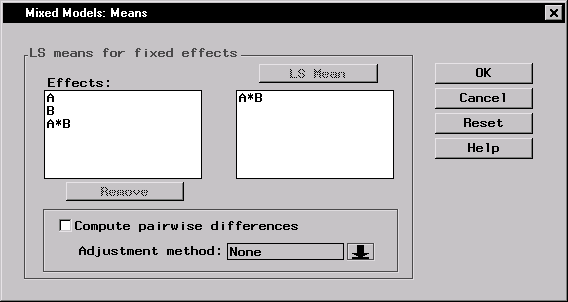Figure 15.4: Mixed Models: Means Dialog

When you have completed your selections, click OK in the main dialog to perform the analysis.

Review the Results

The results are presented in the project tree under the Mixed Models folder, as displayed in Figure 15.5. The two nodes represent the mixed models results and the SAS programming statements (labeled Code) that generate the output.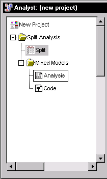

Figure 15.5: Mixed Models: Project Tree

Double-click on the Analysis node in the project tree to view the contents in a separate window.

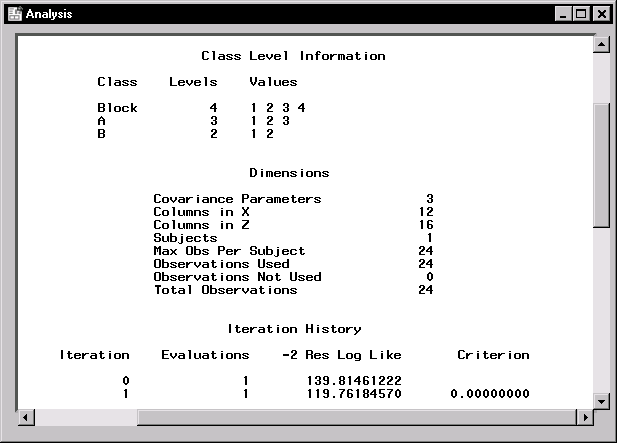Figure 15.6: Mixed Models: Model Information

Figure 15.6 displays class level information, dimensions of model matrices, and the iteration history of the estimated model. The "Class Level Information" table lists the levels of all classification variables included in the model. The "Dimensions" table includes the number of estimated covariance parameters as well as the number of columns in the X and Z design matrices.

The Mixed Models task estimates the variance components for Block, A*Block, and the residual by a method known as residual (restricted) maximum likelihood (REML). The REML estimates are the values that maximize the likelihood of a set of linearly independent error contrasts, and they provide a correction for the downward bias found in the usual maximum likelihood estimates.

The "Iteration History" table records the steps of the REML optimization process. The objective function of the process is -2 times the restricted likelihood. The Mixed Models task attempts to minimize this objective function via the Newton-Raphson algorithm, which uses the first and second derivatives of the objective function to iteratively find its minimum. For this example, only one iteration is required to obtain the estimates. The Evaluations column reveals that the restricted likelihood is evaluated once for each iteration, and the criterion of 0 indicates that the Newton-Raphson algorithm has converged.

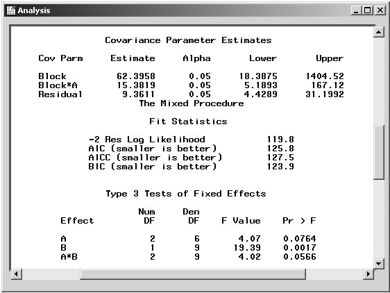Figure 15.7: Mixed Models: Covariance Estimates and Tests for Fixed Effects

Figure 15.7 displays covariance parameter estimates, information on the model fit, and Type 3 tests of fixed effects. The REML estimates for the variance components of Block, A*Block, and the residual are 62.4, 15.4, and 9.4, respectively. The "Fit Statistics" table lists several pieces of information about the fitted mixed model: the -2 residual log likelihood, Akaike's Information Criterion (AIC), a corrected form of AIC that adjusts for small sample size (AICC), and Schwarz's Bayesian Information Criterion (BIC). The information criteria can be used to compare different models; models with smaller values for these criteria are preferred.

The tests of fixed effects are produced using Type 3 estimable functions. The test for the A*B interaction has a p-value of 0.0566, indicating that there is moderate evidence of an interaction between crop varieties and irrigation levels.

Figure 15.8: Mixed Models: Least Squares Means

Figure 15.8 displays the least-squares means for each combination of irrigation levels (A) and crop varieties (B). At each irrigation level, the response is higher for the first crop variety compared to the second variety. The interaction between crop variety and irrigation levels is evident in that variety 1 has a higher mean response than variety 2 at irrigation levels 1 and 2, but the two varieties have nearly the same mean response at irrigation level 3.

Top of Page