Analysis of Variance

Linear Models

The Linear Models task enables you to perform an analysis of variance when you have a continuous dependent variable with classification variables, quantitative variables, or both.

The data set Air, described in the section "The Air Quality Data Set," includes quantitative measures; for example, the variable wind represents wind speed, in knots. Suppose that you want to model ozone levels using the variables day (day of week), shift (factory workshift period), and wind (wind speed). Suppose that you also want your model to include the interaction between the variables day and shift. That is, you want to perform a simple two-way analysis of covariance with unequal slopes.

The following example fits this linear model and additionally requests a retrospective power analysis and a plot of the observed values versus the predicted values.

Request the Linear Models Analysis

To request the linear models analysis, follow these steps:

Select Statistics ANOVA Linear Models ...
Select o3 as the dependent variable.
Select shift and day as the class variables.
Select wind as the quantitative variable.

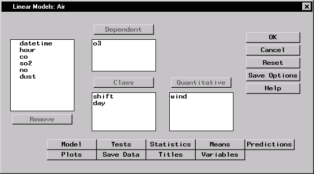Figure 10.19: Linear Models Dialog

Figure 10.19 displays the Linear Models dialog. By default, the linear model analysis includes only the main effects specified in the main dialog: no interaction term is included.

Specifying an Interaction Term in the Model

To include the interaction term shift*day in your model, follow these steps:

Click on the Model button in the main dialog.
Highlight the variables shift and day.
Click on the Cross button.
Click OK.

Note that you can build specific models with the Add, Cross, and Factorial buttons, or you can select a model by clicking on the Standard Models button and making a selection from the pop-up list.

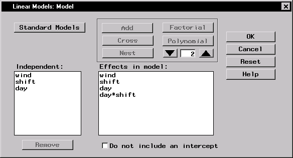Figure 10.20: Linear Models: Model Dialog

Figure 10.20 displays the Model dialog with the terms shift and day and the interaction term shift*day selected as effects in the model.

Request a Power Analysis

The power of a test is the probability of correctly rejecting the null hypothesis of no difference. It depends on the sample size as well as the precise difference specified in the alternative hypothesis. Ideally, you consider power before gathering data to ensure that you gather enough data to detect a difference. However, once you have gathered your data, you can perform a retrospective power analysis in order to determine how much data is needed to detect the observed difference. To perform a retrospective power analysis with the Analyst Application, follow these steps:

Click on the Tests button in the main dialog.
Click on the Power Analysis tab.
Select Perform power analysis.

To request power calculations for tests performed at several $\alpha$ values, you can enter the values, separated by a space, in the box labeled Alphas. You can request power analysis for additional sample sizes in the Sample sizes box. You can enter one or more specific values for the sample sizes, or you can specify a series of sample sizes in the boxes labeled From:, To:, and By:.

Click OK.

Figure 10.21 displays the Power Analysis tab, which requests a retrospective power analysis with an alpha, or significance level, of 0.05.

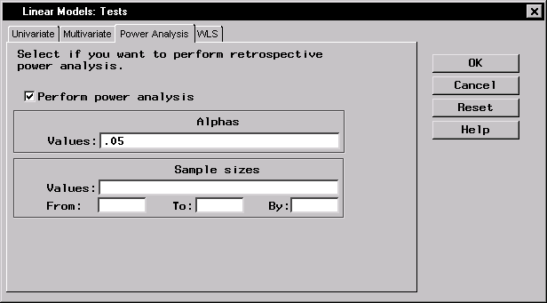Figure 10.21: Linear Models: Tests Dialog

Request a Scatter Plot

To request a scatter plot of the predicted values versus the observed values, follow these steps:

Click on the Plots button in the main dialog.
Click on the Predicted tab.
Select Plot observed vs predicted.
Click OK.

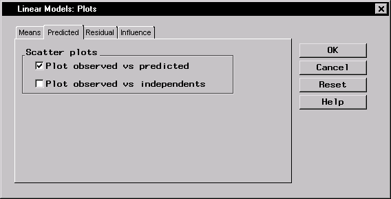Figure 10.22: Linear Models: Plots Dialog

Figure 10.22 displays the Predicted tab in the Plots dialog.

Click OK in the Linear Models dialog to perform the analysis.

Review the Results

The output of the analysis includes information about the levels of the independent variables, followed by the ANOVA table.

Figure 10.23 displays the analysis of variance table, with an F statistic of 19.44 and an associated p-value less than 0.0001. A p-value this small indicates that the model explains a highly significant proportion of the variation in the dependent variable.

The R-square value represents the proportion of variability accounted for by the independent variables. In this analysis, about 74% of the variation of the ozone level can be accounted for by the model (that is, by mean differences in day and shift, in conjunction with a linear dependence on wind speed).

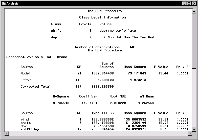Figure 10.23: Linear Models: ANOVA Results

The last table displayed in Figure 10.23 partitions the model sum of squares into the separate contribution for each model effect and tests for the significance of each effect. The main effects and the interaction term are significant at the $\alpha = 0.05$ level (that is, each p-value is less than 0.05).

Figure 10.24 displays the retrospective power analysis. The observed power is given for each effect in the linear model.

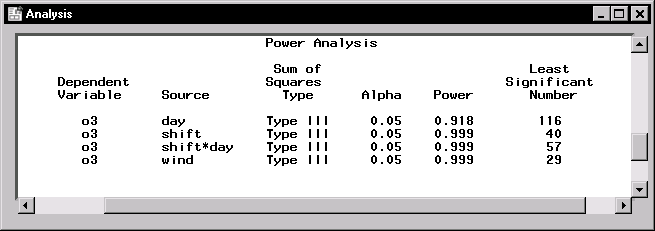Figure 10.24: Linear Models: Power Analysis

The column labeled Least Significant Number in Figure 10.24 displays the smallest number of observations required to determine that the effect is significant at the given $\alpha$ value.

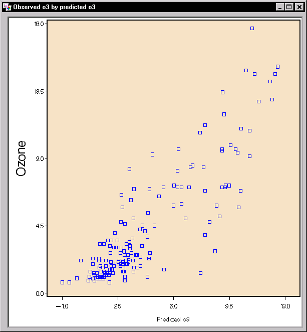Figure 10.25: Linear Models: Observed Ozone Levels versus Predicted Values

Figure 10.25 displays the plot of the observed values versus the predicted values from the model. If the model predicts the observed values perfectly, the points on the plot fall on a straight line with a slope of 1. This plot indicates reasonable prediction.

Top of Page