Analysis of Variance

Factorial Analysis of Variance

The Factorial ANOVA task enables you to perform an analysis of variance when you have multiple classification variables.

For example, consider the data set on air quality (Air), described in the section "The Air Quality Data Set." Suppose you want to compare ozone levels for each day of the week and for each factory workshift. You can define a factorial model that includes the two classification variables, day and shift.

In this example, a factorial model is specified, and a plot of the two-way effects is requested.

Request the Analysis

To request a factorial analysis of variance, follow these steps:

Click on Statistics ANOVA Factorial ANOVA ...
Select o3 as the dependent variable.
Select shift and day as the independent variables.

The resulting Factorial ANOVA dialog is displayed in Figure 10.14.

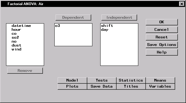Figure 10.14: Factorial ANOVA Dialog

The default ANOVA model includes only the main effects (that is, the terms representing shift and day). To include an interaction term, or to specify other options for your analysis, you can use the dialogs available in the Factorial ANOVA task.

Specify the Model

To specify a factorial model, follow these steps:

Click on the Model button in the main dialog.
Highlight the variables shift and day in the resulting dialog.
Click on the Factorial button.
Click OK.

Figure 10.15 displays the Model dialog with the terms shift, day, and the interaction term shift*day selected as effects in the model.

Note that you can build specific models with the Add, Cross, and Factorial buttons, or you can select a model by clicking on the Standard Models button and making a selection from the drop-down list. From this list, you can request that your model include main effects only, effects up to two-way interactions, or effects up to three-way interactions.

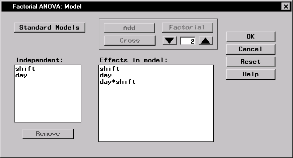Figure 10.15: Factorial ANOVA: Model Dialog

Request a Means Plot

A means plot displays a symbol for the observed or predicted means at each level of a specified variable, with vertical bars extending for a specified number of standard errors. The means for each level of an effect are joined with line segments. To request a plot of the dependent means, follow these steps:

Click on the Plots button in the main dialog. The resulting window displays the Means tab.
Select Plot dependent means for two-way effects.

You can choose to plot either the observed or predicted means of the dependent variable. Additionally, you can choose whether the vertical bars should represent one, two, or three standard errors.

Click OK.

Figure 10.16 requests a plot of the observed dependent means for the two-way effects.

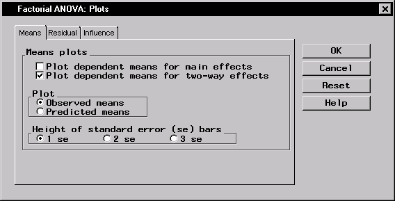Figure 10.16: Factorial ANOVA: Plots Dialog

Click OK in the main dialog to perform the analysis.

Review the Results

Figure 10.17 displays information on the levels of the two classification variables, shift and day, followed by the ANOVA table. The model sum of squares is partitioned into the separate contributions of the individual model effects, and F tests are provided for each effect.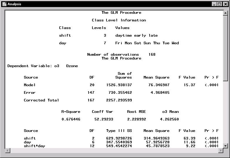

Figure 10.17: Factorial ANOVA: Analysis Results

The F statistic of 15.37 indicates that the model as a whole is highly significant (the p-value is less than 0.0001). Additionally, the R-square value of 0.6764 means that about 68% of the variation of ozone can be accounted for by the factorial model.

The table at the bottom of Figure 10.17 displays the significance test for each term of the model. The main effects and the interaction term are each significant at the $\alpha = 0.05$ level (that is, each p-value is much less than 0.05).

In Figure 10.18, the three curves display ozone concentration across days of the week. Each curve represents the relationship for one of the three factory workshift periods.

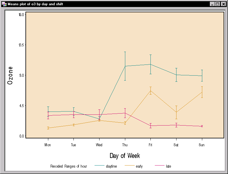Figure 10.18: Factorial ANOVA: Means Plot

The means plot indicates an inverse relationship between the daytime and late shifts. The ozone levels during the daytime shift rise dramatically on Thursday and remain high throughout the weekend. Ozone levels for the late shift, on the other hand, start to decrease after Thursday and remain low throughout the weekend.

Top of Page