SAS Products
SAS Risk Dimensions - Using Distortion Risk Measures
Specify the Analysis and Create the Project
Overview
Risk measures help us understand how data is distributed. A commonly consulted risk measure is expected value, which helps us understand what happens on average. As informative as expected value can be, it can fail to convey the full risk picture. For example, consider two scenarios. In the first, you get $0 with 100% certainty. In the second, you lose $100 50% of the time and win $100 50% of the time. Both scenarios have an expected value of $0, but the second is considerably riskier with regard to loss. We need other risk measures to better understand the occurrence and magnitude of loss.
That is where distortion risk measures prove useful. A distortion risk measure provides the expected value of a probability distribution after it has been altered with a distortion function. Distortion functions essentially re-weight a distribution to put more emphasis on particular outcomes. For example, value at risk (VaR) is a distortion risk measure. The VaR distortion function puts all of the weight on the occurrence of loss at a given percentile and puts no weight on the other outcomes. Conditional value at risk (CVaR) is also a distortion risk measure. Its distortion function assigns equal weights to all loss outcomes worse than a given percentile and zero weight to all other outcomes.
Some common distortion risk measures, including VaR and CVaR, are provided by SAS Risk Dimensions. You can define others and register them in a risk environment.
Objective
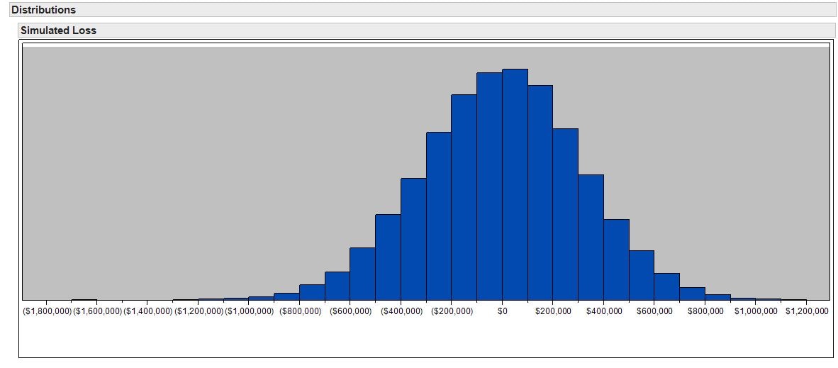
Suppose you simulate the value of a portfolio that contains two shares of stock (see "Assessing Market Risk" for more information about this simulation). You generate 50,000 market states and calculate the portfolio's value and profit/loss at each market state.
The following figure shows the distribution of simulated losses.
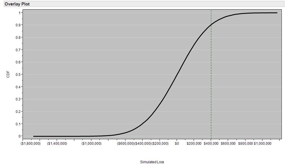
This loss distribution has the corresponding cumulative distribution function (CDF) plotted below. This figure shows the probability that the portfolio loss will be less than or equal to the value on the x-axis. For example, approximately 90% of the losses will be less than $400,000, which means that approximately 10% of the losses will exceed $400,000.
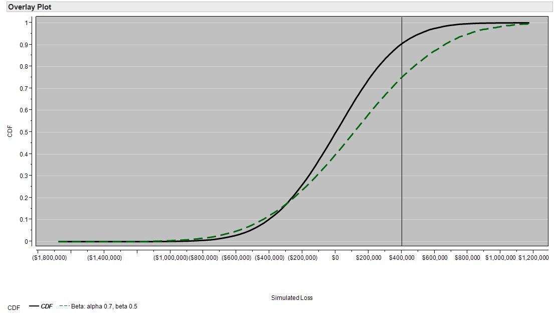
When you use distortion functions to assess risk, you re-weight the distribution to emphasize unfavorable outcomes. The figure below shows the application of the beta distortion function to the CDF. With this transformation, there is now a ~25% chance that the loss exceeds $400,000. The expected loss of the distorted distribution is $107,939 versus the $3,167 expected loss of the original distribution
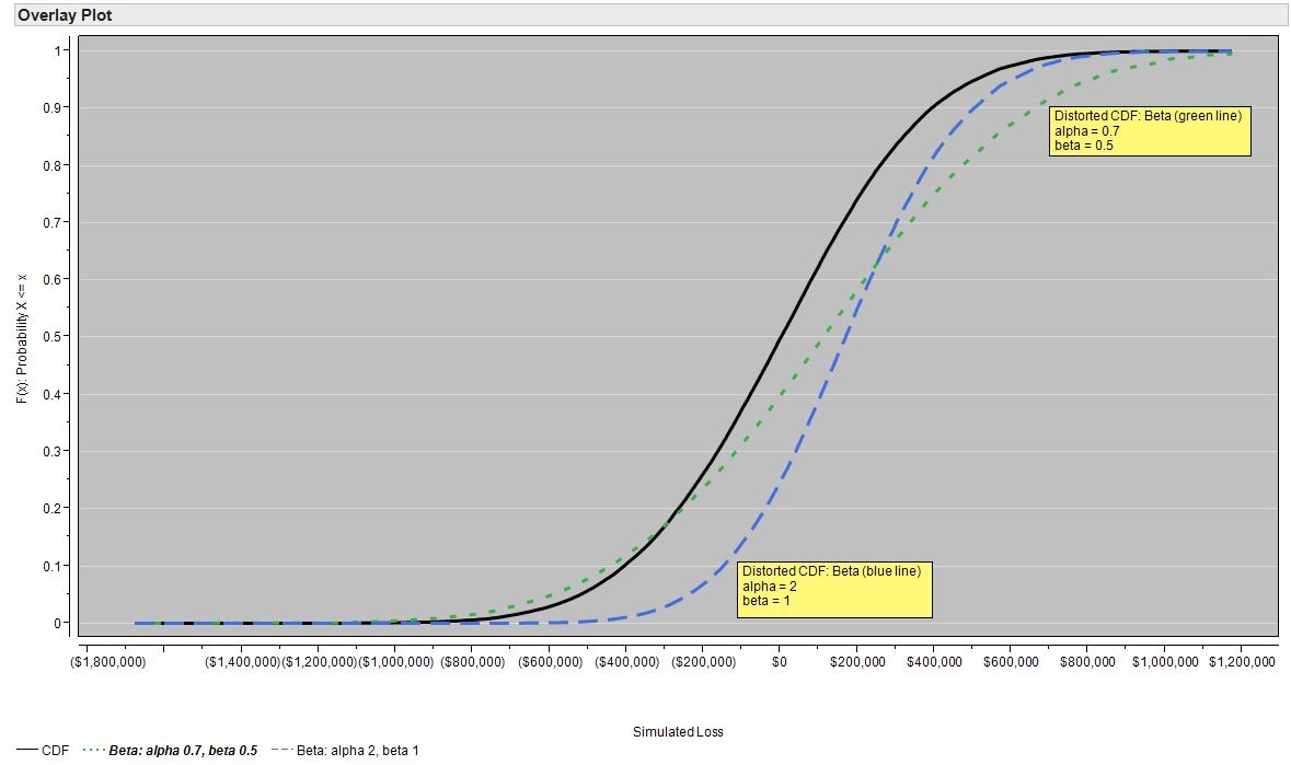
Different distortion functions distort the CDF in different ways. Further, most distortion risk measures have parameters that affect how the CDF is distorted. For example, by varying the alpha and beta parameters in the beta distortion function, you can choose the type of losses to emphasize.
In the following figure, the beta distortion function illustrated by the green line gives heavier weight to losses greater than $200,000 while the beta distortion function illustrated by the blue line gives more weight to losses less than $200,000.
In the following example, you apply the beta distortion function with an alpha parameter of 0.7 and a beta parameter of 0.5. Because this distortion function is not provided with SAS Risk Dimensions, you need to define it in your environment. For comparison, you examine two familiar built-in distortion risk measures, value at risk (VaR) and conditional value at risk (CVaR).
Set Up the Environment
First, set up the library for analysis and the name of the SAS Risk Dimensions environment. Use the directory C:\users\sasdemo\RD_Examples. You can assign the libref to any path as long as you have Write access to that directory.
%let test_env = distortionmeasures;
In this code, you use the SAS Macro Language Facility to create the macro variable test_env. You assign the value distortionmeasures to the variable test_env. Using macro variables in this way gives you the flexibility to change the physical location of the target library and environment name in just two lines of code.
Next, create a new SAS Risk Dimensions environment assigned the name distortionmeasures in the library RDExamp.
env save;
Register Your Portfolio Data
Next, describe the assets in your portfolio. . The following code creates a data set called instdata that stores information about the two instruments in your portfolio. Use the RISK procedure to register three instrument variables: InstType, InstID, and Holding.
datalines;
BankCompany instid2 1000000
;
instdata Instruments file=RDExamp.instdata format=simple;
env save;
Register Market Data
There are two risk factors, TEC and BNK, which represent the prices of TechCompany stock and BankCompany stock. Define the current risk factor values and covariances. Declare the risk factors and register the market data in the environment.
BNK=30;
_type_ = "COV";
input _name_ $ TEC BNK;
datalines;
BNK .00006 .0001
;
declare riskfactors=(TEC num var, BNK num var);
marketdata Market file=RDExamp.mktdata type=current;
marketdata Cov file=RDExamp.covdata type=covariance;
env save;
Define Valuation Methods
Create pricing methods using the COMPILE procedure for use in this environment. The COMPILE procedure is similar to and supports the functionality and syntax of the FCMP procedure. For more information, see the SAS Risk Dimensions: Users Guide.
Tell the RISK procedure which pricing methods to use for each of the instrument types through assignment in the INSTRUMENT statement. Also specify the instrument variables needed for pricing; insttype and instid do not need to be specified as they are included by default. In addition to the pricing methods, define the distortion function, BetaDistortion. This function is used to compute the beta distortion risk measure. When you define a distortion function, you must include the parameter x, which is the value of the empirical cumulative distribution function.
_value_ = TEC;
endmethod;
method Bank_Price kind=price;
_value_ = BNK;
endmethod;
instrument TechCompany methods=(Price Tech_Price)variables = (holding);
instrument BankCompany methods=(Price Bank_Price)variables = (holding);
env save;
Specify the Analysis and Create the Project
Set up a project to simulate values for your portfolio based on the current market data and the covariance data. Use the DISTORTION statement to specify distortion risk measures. The distortion risk measures are output to the SimStat data set.
sources InstDataSource (Instruments);
read sources=InstDataSource out=Portfolio;
crossclass InstTypeCC (Insttype);
simulation Covariance method=covariance
outvars=(pl)
portfolio=Portfolio
crossclass=InstTypeCC
data=( Market )
;
Run the Project
Run the project, putting output files in the DistOut subdirectory of the environment.
setoptions keeplib;
runproject Project
options=( outall)
;
View Results
Next, analyze your results. You can perform analysis on SAS data sets output from the project.
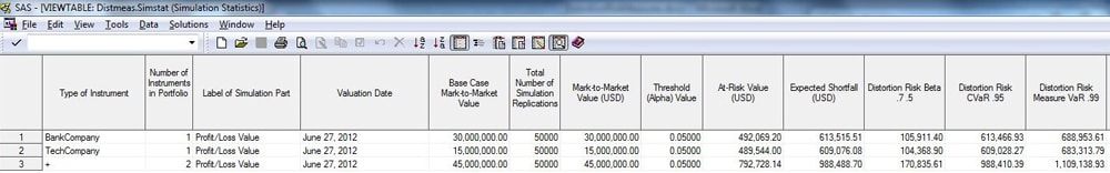
The following figure shows the SimStat data set generated by the project run. The distortion risk measures specified in the environment appear in the data set.