Usage Note 71200: Find optimal cutpoints and area (AUC) for ROC and precision-recall curves from a binary response model
 |  |  |
In SAS® 9, optimal cutpoints on the Receiver Operating Characteristic (ROC) curve, using any of several criteria, can be found using the ROCPLOT macro (SAS Note 25018). Similarly, for the precision-recall (PR) curve, cutpoints that are optimal on the F and MCC criteria can be identified using the PRcurve macro (SAS Note 68077). Both macros can be used after fitting a binary response model in PROC LOGISTIC with the OUTROC= option to create a data set of points on the ROC curve.
In SAS® Viya®, options are available in PROC LOGISTIC that can plot both the ROC and PR curve (using any of several methods) and can identify optimal cutpoints on these curves.
As discussed in the PRcurve macro documentation, the ROC curve and the area under it (AUC) can be misleading when the proportions of events and nonevents become very imbalanced, such as when there are very few observed events. In these cases, the PR curve and its AUC provide a better assessment. The PR curve is a remapping of the ROC curve.
Some examples of using the PRcurve macro can be found in the macro documentation at the link above. In addition to showing use of the macro, the examples also show equivalent use of the options available in PROC LOGISTIC in SAS Viya. The following provides additional examples of using both.
Example 1: Optimal cutpoints on ROC and PR Curves
An example of plotting the ROC and PR curves and identifying optimal cutpoints appears in the example titled "Using the Optimal ROC Criteria" in the SAS Viya documentation of PROC LOGISTIC. Note that this SAS Viya example uses the binormal method to estimate both curves, which is one of the methods available. Another available method is METHOD=LOWER. It is this method that the macros use. This method typically produces a plot that is more jagged in appearance than the smoothed plot from METHOD=BINORMAL, which assumes that the predicted probabilities are normally distributed.
The following modifies the documentation example to create the curves using METHOD=LOWER in PROC LOGISTIC and produces the same results with the PRcurve macro. First, statements producing the PR curve and optimal points using PROC LOGISTIC in SAS Viya are shown. Note the use of the ID statement so that the model predictors are added in the OUTROC= data set and can be used to identify the optimal points. The added variables _OPTF1_, _OPTMCC_, and _OPTYOUDEN_ are 0,1 indicators that are set to 1 when the observation is the optimal cutpoint on the F, MCC, and Youden criteria. The added variables _F_, _MCC_, and _YOUDEN_ are the values of those criteria:
   proc logistic data=Mroz plots(only)=(roc pr) rocoptions(method=lower optimal=(f mcc youden));
      model InLaborForce2(event='0') = IncomeExcl Education Experience SqExperience
            Age KidsLt6 KidsGe6 / outroc=outr;
      id IncomeExcl Education Experience SqExperience Age KidsLt6 KidsGe6;
      run;
   proc print data=outr(where=(_optmcc_=1 or _optf1_=1 or _optyouden_=1)) noobs;
      id IncomeExcl Education Experience SqExperience Age KidsLt6 KidsGe6;
      var _prob_ _opt: _f1_ _mcc_ _youden_;
      title "Optimal Cutpoints";
      run;
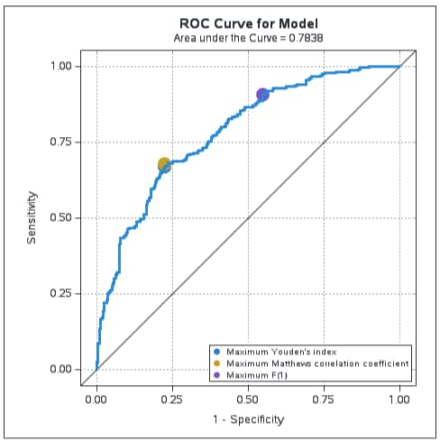
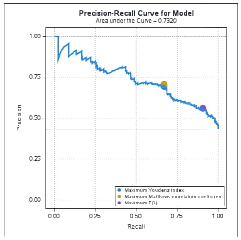
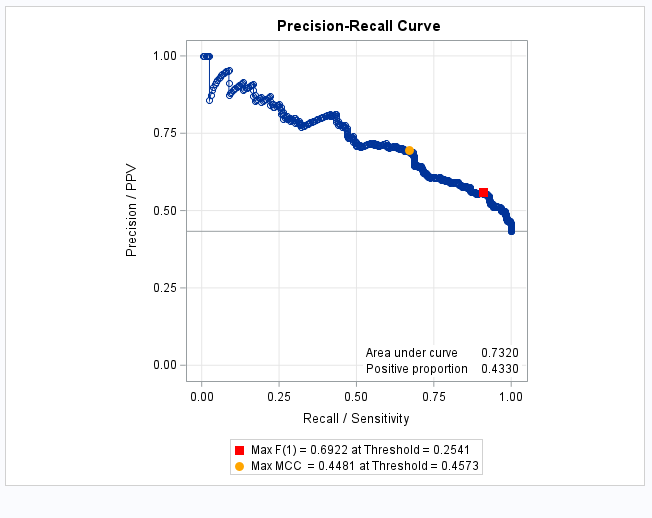
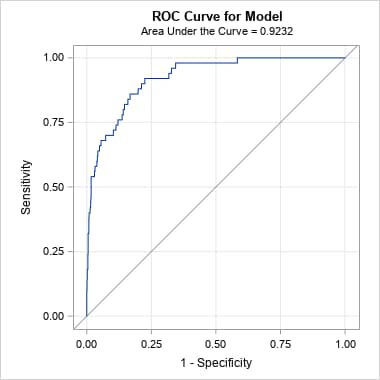
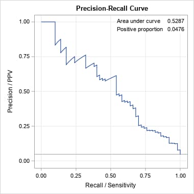
The ROC and PR curves are shown below. Since the proportions of events and nonevents are not badly unbalanced in this data set, the ROC and PR curves provide similar assessments of the model as reflected by similarity of the areas beneath them.
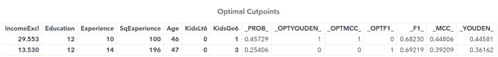
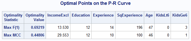
In the first observation in the Optimal Cutpoints table, the _OPTYOUDEN_ and _OPTMCC_ variables indicate that 0.45729 is the optimal cutpoint on the probability scale for both criteria. The value of the Youden criterion at that point is 0.44581 and 0.44806 is the value of the MCC criterion. The values related to the optimal cutpoint on the F1 criterion are shown in the second observation. The variables from the ID statement identify each point in terms of the model predictors:
   |
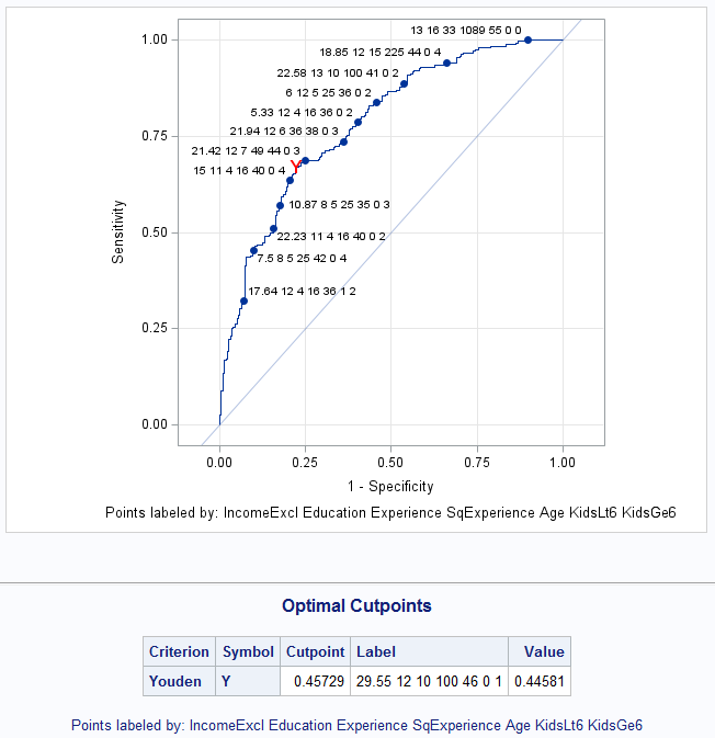
While the ROCPLOT macro does not offer the F and MCC criteria, it does offer most of the other criteria available in PROC LOGISTIC. The following shows use of the ROCPLOT macro to identify the cutpoint optimal on the Youden criterion. This point is highlighted in the plot and provided in a table, which includes the identifying predictor values. Note the use of the OUTPUT statement to obtain a copy of the input data set with the predicted event probabilities added. This is needed in the ROCPLOT macro. It is also needed in the PRcurve macro if optvars= is specified:
   proc logistic data=Mroz;
      model InLaborForce2(event='0') = IncomeExcl Education Experience SqExperience
            Age KidsLt6 KidsGe6 / outroc=outr;
      output out=logpred p=pred;
      run;
   %rocplot(inroc=outr, inpred=logpred, p=pred, optcrit=youden,
      id=IncomeExcl Education Experience SqExperience Age KidsLt6 KidsGe6,
      optsymbolstyle=size=12 color=red weight=bold)
Notice that the same Youden-optimal point is identified at the same probability and criterion values as above:
 |
Finally, the following shows the equivalent use of the PRcurve macro specifying inpred=, pred=, and optvars= to display a table showing the optimal points and associated predictor values:
   %prcurve(data=outr, options=optimal, inpred=logpred, pred=pred,
      optvars=IncomeExcl Education Experience SqExperience Age KidsLt6 KidsGe6)
The PR curve is the same as from PROC LOGISTIC above and the same optimal points are identified for the F and MCC criteria. Note also that the area under the PR curve, 0.7320, is the same as from PROC LOGISTIC:
  |
Example 2: Compare ROC and PR Curves with Balanced and Unbalanced Data
This example illustrates the invariance of the ROC curve to the level of imbalance among events and nonevents in the data. This invariance makes the ROC curve and area under it (AUC) misleading in cases where the imbalance is strong, such as when the event is rare in the population.
The following statements generate balanced and unbalanced data sets with a predictor, X, that moderately separates the events and nonevents. The balanced data set contains 2,000 observations with equal numbers of events and nonevents. Another data set of 2,000 observations is created in which only 5% of the observations are events:
    data bal;
      do i=1 to 1000; y=1; x=rannor(2315)+0.5; output; end;
      do i=1 to 1000; y=0; x=rannor(2315); output; end;
      run;
    data unbal;
      do i=1 to 50;   y=1; x=rannor(2315)+0.5; output; end;
      do i=1 to 1000; y=0; x=rannor(2315); output; end;
      run;
These statements fit the model to the balanced data and produce the ROC and PR curves. The nomarkers option is used since there are a large number of points in the OUTROC= data sets. The tr option is used to move the positive proportion and area information to the top right corner of the plot:
To obtain the plots in SAS Viya, add PLOTS(ONLY)=(ROC PR) in the PROC LOGISTIC statement rather than use the PRcurve macro:
    proc logistic data=bal;
      model y(event="1")=x / outroc=or;
      run;
    %prcurve(options=nomarkers tr)
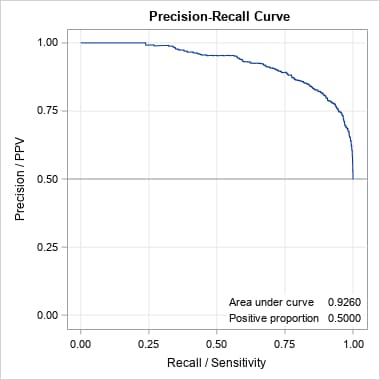
Following are the curves produced by the PRcurve macro. Note that for these balanced data, both curves and the areas under them give similar results. Both suggest moderate model performance.
 |
 |
These statements fit the model to the unbalanced data:
    proc logistic data=unbal;
      model y(event="1")=x / outroc=or;
      run;
    %prcurve(options=nomarkers tr)
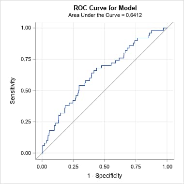
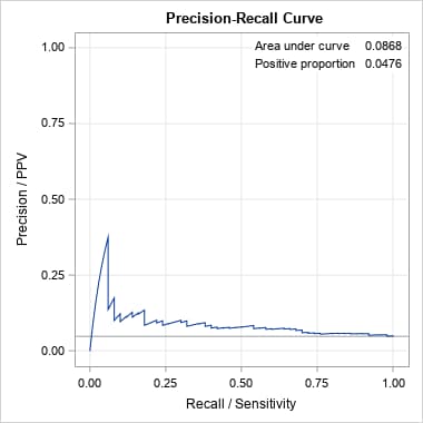
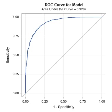
Following are the curves produced by the PRcurve macro. For the unbalanced data, note that the ROC curve and AUC are little changed. However, the PR curve differs dramatically from the PR curve for the balanced data, and the AUC has dropped from 0.63 to 0.09. That is because the precision (or positive predictive value, PPV) at each threshold on the predicted probabilities is very low. That is, the probability at each threshold of a predicted event being an actual event is low in the unbalanced data. This information is not captured by the ROC curve:
 |
 |
Next, balanced and unbalanced data sets are generated with the predictor providing good separation between events and nonevents. As before, both data sets contain 2,000 observations with 50% events in the balanced data set and only 5% events in the unbalanced data set:
    data bal;
      do i=1 to 1000; y=1; x=rannor(2315)+2; output; end;
      do i=1 to 1000; y=0; x=rannor(2315); output; end;
      run;
    data unbal;
      do i=1 to 50;   y=1; x=rannor(2315)+2; output; end;
      do i=1 to 1000; y=0; x=rannor(2315); output; end;
      run;
These statements produce the ROC and PR curves and areas:
    proc logistic data=bal;
      model y(event="1")=x / outroc=or;
      run;
    %prcurve(options=nomarkers)

    proc logistic data=unbal;
      model y(event="1")=x / outroc=or;
      run;
    %prcurve(options=nomarkers tr)
As before, to obtain the plots in SAS Viya, add PLOTS(ONLY)=(ROC PR) in the PROC LOGISTIC statement rather than use the PRcurve macro.
Again, the ROC and PR curves and AUCs give similar results when the data are balanced, but even in this case with relatively well-separated event and nonevent populations, the two curves give very different assessments of the model performance in the unbalanced data. The ROC curve and AUC are essentially unchanged, missing the much lower proportions of true positives among the predicted positives in the unbalanced data. The PR curve reveals those lower proportions, particularly at the moderate and higher sensitivities occurring at lower thresholds on the predicted probabilities. The reduced AUC value summarizes this decrease in performance.
 |
 |
 |
 |
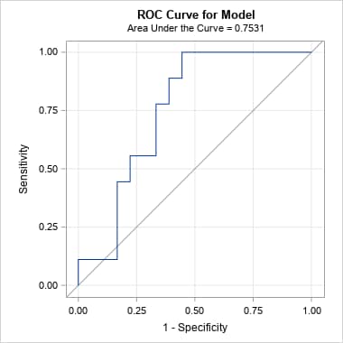
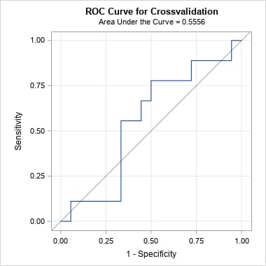
Example 3: Cross-validated Precision-recall Curve
The following uses the cancer remission data in the example titled "Stepwise Logistic Regression and Predicted Values" in the PROC LOGISTIC documentation. The PRcurve macro can produce a cross-validated PR curve by using the data from the CTABLE option in PROC LOGISTIC. That option uses an approximate leave-one-out cross-validation method to produce classification table statistics over a range of thresholds on the predicted probabilities. Cross validation reduces the bias that results from using the same data to both fit the model and assess its performance.
In SAS Viya, cross-validated ROC and PR curves can be obtained by adding the PLOTS(ONLY)=(ROC PR) and ROCOPTIONS(CROSSVALIDATE) options in the PROC LOGISTIC statement. In SAS®9, the ROCOPTIONS(CROSSVALIDATE) option can also be used to produce the cross-validated ROC curve only. To obtain the cross-validated PR curve using the PRcurve macro, save the table produced by the CTABLE option and specify it as the data= data set in the PRcurve macro.
In SAS Viya, the first PROC LOGISTIC step below produces the ROC and PR curves without cross-validation using the default empirical method. The second step produces the cross-validated curves:
    proc logistic data=remission plots(only)=(roc pr);
       model remiss(event='1') = smear blast;
       run;
    proc logistic data=remission plots(only)=(roc pr) rocoptions(crossvalidate);
       Crossvalidation: model remiss(event='1') = smear blast;
       run;
Equivalently, the first PROC LOGISTIC step and PRcurve macro call below fit the logistic model and produce the ROC and PR curves without cross-validation. The second PROC LOGISTIC step and PRcurve macro call produce the cross-validated curves. Creating ROC curves using both validation and cross validation is further discussed in SAS Note 39724.
    proc logistic data=remission;
       model remiss(event='1') = smear blast / outroc=remor;
       run;
    %prcurve(data=remor)

    proc logistic data=remission rocoptions(crossvalidate) plots(only)=roc;
       Crossvalidation: model remiss(event='1') = smear blast / ctable;
       ods output classification=remct;
       run;
    %prcurve(data=remct)
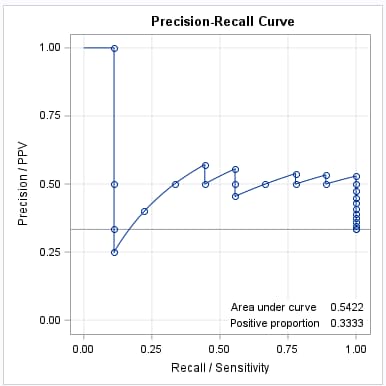
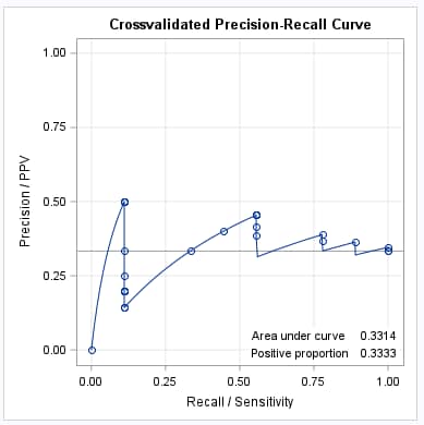
Following are the curves, with and without cross-validation, produced by the PRcurve macro. Notice that the cross-validated ROC curve on the right has substantially reduced area from the ordinary ROC curve on the left. That reflects the effect of removing the optimistic bias resulting from using the training data to assess the model.
 |
 |
Similar to the ROC curves, the cross-validated PR curve has lower area as a result of the bias-reducing cross-validation method.
 |
 |
Example 4: Precision-recall Curve for Validation Data
The following continues the example in SAS Note 39724, which illustrates obtaining the ROC curve for applying a fitted model to a separate data set for validation. The following statements produce both the ROC and PR curves for the training and the validation data sets.
These statements produce ROC curves for both training and validation data using PROC LOGISTIC and then the PR curves for both data sets using the PRcurve macro. Using SAS Viya, the PRcurve macro calls can be omitted by adding the PLOTS(ONLY)=(ROC PR) option and the ROCOPTIONS(METHOD=LOWER) option, or your choice of method, in the PROC LOGISTIC statement. Slight differences in plotted points and area under the PR curves are due to the procedure in SAS Viya and the macro choosing different sets of points in the interpolation process. But any set of points provides a valid estimate of the curve.
   proc logistic data=train;
      model y(event="1") = entry / outroc=troc;
      score data=valid out=valpred outroc=vroc;
      run;
   %prcurve(data=troc)
   %prcurve(data=vroc)
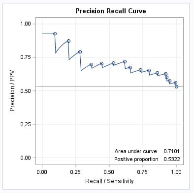
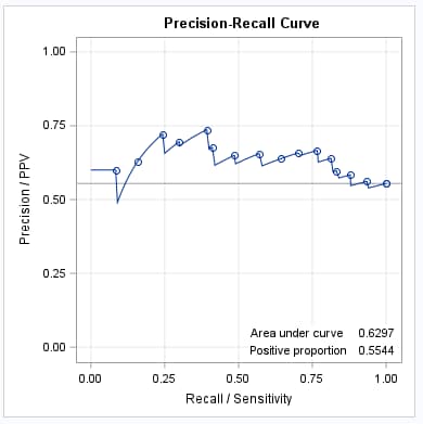
Following are the PR curves for the training (left) and validation (right) data sets as produced by the PRcurve macro. Note the lower AUC value, from 0.71 to 0.63, which results from the use of separate data to provide a better, less biased, assessment of the model. Also note that these AUC values for the PR curves are similar to those for the ROC curves shown in the above note because the data do not exhibit strong imbalance of events and nonevents.
 |
 |
Operating System and Release Information
| Product Family | Product | System | SAS Release | |
| Reported | Fixed* | |||
| SAS System | SAS/STAT | z/OS | ||
| z/OS 64-bit | ||||
| OpenVMS VAX | ||||
| Microsoft® Windows® for 64-Bit Itanium-based Systems | ||||
| Microsoft Windows Server 2003 Datacenter 64-bit Edition | ||||
| Microsoft Windows Server 2003 Enterprise 64-bit Edition | ||||
| Microsoft Windows XP 64-bit Edition | ||||
| Microsoft® Windows® for x64 | ||||
| OS/2 | ||||
| Microsoft Windows 8 Enterprise 32-bit | ||||
| Microsoft Windows 8 Enterprise x64 | ||||
| Microsoft Windows 8 Pro 32-bit | ||||
| Microsoft Windows 8 Pro x64 | ||||
| Microsoft Windows 8.1 Enterprise 32-bit | ||||
| Microsoft Windows 8.1 Enterprise x64 | ||||
| Microsoft Windows 8.1 Pro 32-bit | ||||
| Microsoft Windows 8.1 Pro x64 | ||||
| Microsoft Windows 10 | ||||
| Microsoft Windows 11 | ||||
| Microsoft Windows 95/98 | ||||
| Microsoft Windows 2000 Advanced Server | ||||
| Microsoft Windows 2000 Datacenter Server | ||||
| Microsoft Windows 2000 Server | ||||
| Microsoft Windows 2000 Professional | ||||
| Microsoft Windows NT Workstation | ||||
| Microsoft Windows Server 2003 Datacenter Edition | ||||
| Microsoft Windows Server 2003 Enterprise Edition | ||||
| Microsoft Windows Server 2003 Standard Edition | ||||
| Microsoft Windows Server 2003 for x64 | ||||
| Microsoft Windows Server 2008 | ||||
| Microsoft Windows Server 2008 R2 | ||||
| Microsoft Windows Server 2008 for x64 | ||||
| Microsoft Windows Server 2012 Datacenter | ||||
| Microsoft Windows Server 2012 R2 Datacenter | ||||
| Microsoft Windows Server 2012 R2 Std | ||||
| Microsoft Windows Server 2012 Std | ||||
| Microsoft Windows Server 2016 | ||||
| Microsoft Windows Server 2019 | ||||
| Microsoft Windows Server 2022 | ||||
| Microsoft Windows XP Professional | ||||
| Windows 7 Enterprise 32 bit | ||||
| Windows 7 Enterprise x64 | ||||
| Windows 7 Home Premium 32 bit | ||||
| Windows 7 Home Premium x64 | ||||
| Windows 7 Professional 32 bit | ||||
| Windows 7 Professional x64 | ||||
| Windows 7 Ultimate 32 bit | ||||
| Windows 7 Ultimate x64 | ||||
| Windows Millennium Edition (Me) | ||||
| Windows Vista | ||||
| Windows Vista for x64 | ||||
| 64-bit Enabled AIX | ||||
| 64-bit Enabled HP-UX | ||||
| 64-bit Enabled Solaris | ||||
| ABI+ for Intel Architecture | ||||
| AIX | ||||
| HP-UX | ||||
| HP-UX IPF | ||||
| IRIX | ||||
| Linux | ||||
| Linux for x64 | ||||
| Linux on Itanium | ||||
| OpenVMS Alpha | ||||
| OpenVMS on HP Integrity | ||||
| Solaris | ||||
| Solaris for x64 | ||||
| Tru64 UNIX | ||||
| Type: | Usage Note |
| Priority: | |
| Topic: | Analytics ==> Categorical Data Analysis Analytics ==> Statistical Graphics SAS Reference ==> Macro |
| Date Modified: | 2025-06-24 15:51:19 |
| Date Created: | 2025-06-17 11:58:49 |